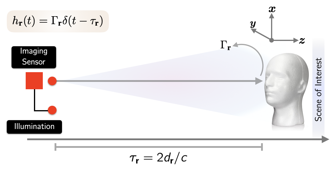
Transient Imaging and the ToF Principle.
Time-of-Flight (ToF) is a consumer-grade 3D imaging technology based on a sensor that can access the transient information of the scene—the reflectivity of an object \(\Gamma_{\mathbf{r}}\), and its distance from the sensor \(z_{\mathbf{r}}\), at location \(\mathbf{r}\).
In the transient image, the reflectivity is encoded as the light intensity, while the distance is encoded in the travel time of the light from the object to the sensor, hence the time-of-flight principle. Mathematically, the transient image is written as \(h_{\mathbf{r}}(t) = \Gamma_{\mathbf{r}}\delta(t-\tau_{\mathbf{r}})\).
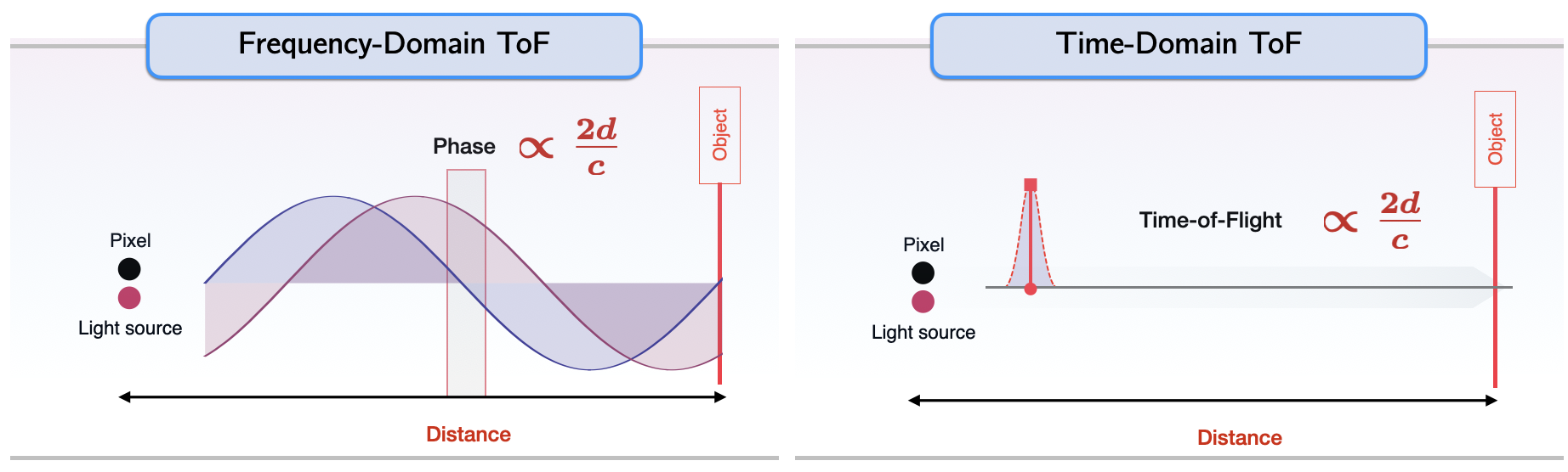
Fourier-domain ToF vs Time-domain ToF.
In the imaging process, the scene is probed using a ray of light, the backscattered signal (or a processed version of it) is sampled over time. Then, algorithms are used to extract the amplitude and distance from samples.
The existing methods can be classified based on the domain of measurement.
Fourier-domain ToF (indirect-ToF):
The scene is probed by a frequency-localized waveform.
The distance is encoded as a frequency-dependent phase.
Time-domain ToF (direct ToF):
The scene is probed by a time-localized waveform.
The distance is encoded as the round trip time of the pulse.
Fig. 27 Comparison of Frequency-Domain ToF and Time-Domain ToF.
Time-of-flight sensors are being used in commercial products for depth imaging and beyond.
Examples are non-line-of-sight imaging and bio-medical uses, where robustness and stability are essential.
Since the backscattered signal amplitudes are recorded by an ADC, saturation is a limiting source.
This affects not only the measured amplitudes, but also contaminate the depth estimation, as this process is performed algorithmically based on the measured intensities.
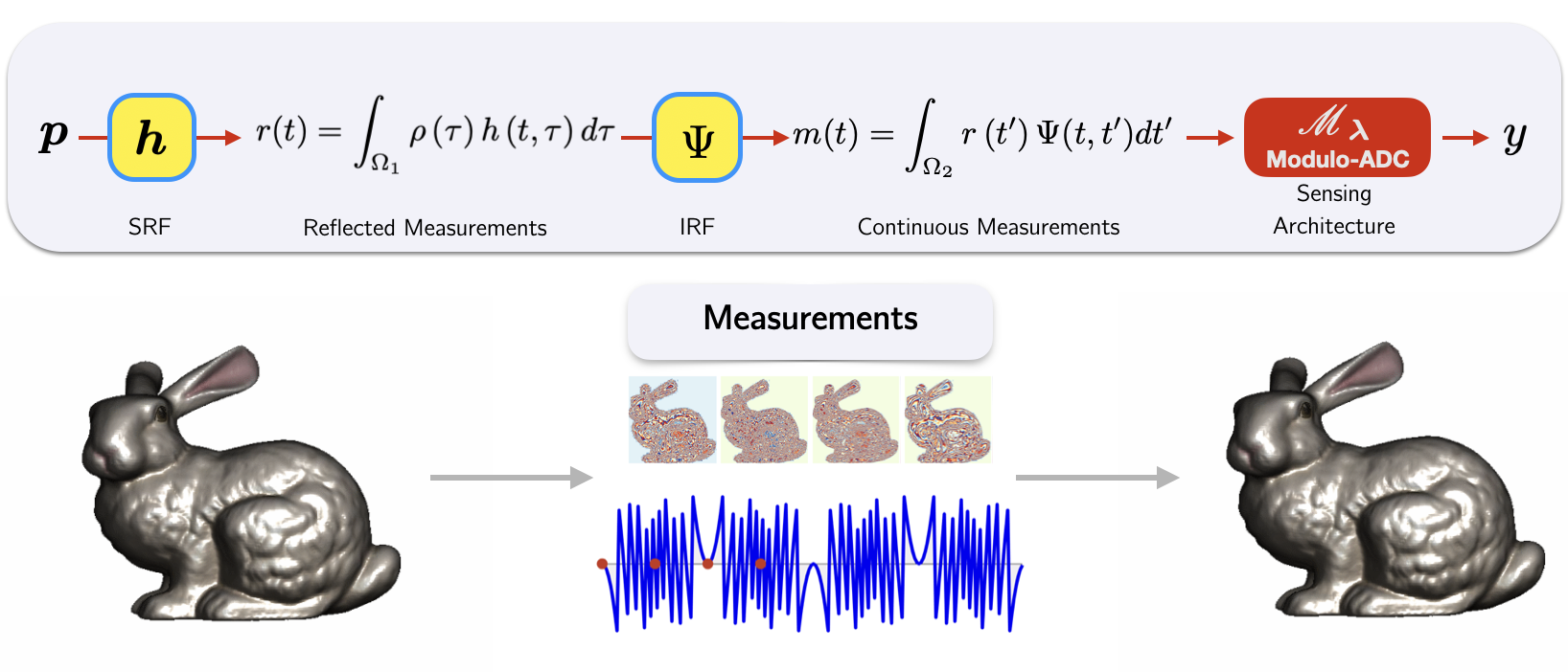
The USF-ToF Acquisition Pipeline Forward Model.
To enable HDR and high-resolution capabilities, the conventional ADC in ToF imaging pipelines is replaced by the M-ADC. The imaging pipeline is illustrated by the next figure.
iToF and dToF architectures differ in their probing function \(p(t)\). In iToF, the scene is probed with a sinusoidal waveform, while in dToF, it is probed by a pulse.
A lock-in sensor cross-correlates the backscattered and the probing signals to generate the measured signal.
The Inverse Problem
Estimating amplitude and depth from modulo measurements poses an inverse problem which depends on the sensing architecture. The USF methods in [1], [3] can first unfold the modulo samples, allowing the use of existing techniques for parameter estimation.
This means using [1] for iToF (where sinusoidal signals are bandlimited) and [3] for dToF.
However, this approach fails to leverage signal priors, leading to suboptimal results.
For each architecture, a solution that directly estimates the parameters has been developed. This minimizes the sampling rate and improves the stability.
In the iToF architecture, the depth and amplitude parameters \((\Gamma,\theta)\), where \(\theta=\omega_{0}\frac{2z}{c}\) and \(c\) is the velocity of light, are traditionally found as the amplitude and phase of a phasor, following the Four Bucket Method.
However, this algorithm can not be used on modulo measurements and modification of the sampling rate and the estimation algorithm is needed.
The approach for modulo-based iToF is based on two observations:
The sinusoidal and residual components of the modulo samples are separable in the higher-order-differences domain.
Sinusoidal are closed under the finite-differences operator, and the frequency and phase parameters can be accessed.
To leverage the first observation, the closed-form equation for the \(N^{\mathrm{th}}\) order differences of the sine function is computed,
\[\left( {{\Delta ^N}{m_{\mathbf{r}}}} \right)\left[ k \right] = {2^N}\left( {{\Gamma _{\mathbf{r}}}\frac{{\rho _0^2}}{2}} \right){\sin ^N}\left( {\frac{{\omega_0 T}}{2}} \right)\cos \left( {k\omega_0 T + \frac{N}{2} (\omega_0 T + \pi) + {\theta _{\mathbf{r}}}} \right).\]
The max-norm of the LHS is bounded as a function of the sampling rate \(T\), and the order \(N\) determines its maximum value.
To leverage the second observation, the desired parameters are isolated in the higher-order-differences domain and a least-square solution is used to estimate them.
Modulo CW-ToF Imaging
Let \(y[k]\) be the modulo samples obtained from a CW-ToF imager, operating at modulation frequency \(\omega_0\). Furthermore, assume that an upper bound \(\beta_\rho^\Gamma \geq \left| \frac{1}{2} \Gamma_\mathbf{r} \rho_0^2 \right|\) is known. Then, the unknown parameters \(\{\Gamma_\mathbf{r}, \theta_\mathbf{r}\}\) can be estimated from \(N + 2\) modulo samples if the sampling time satisfies,
\[T_{\text{ToF}} < \frac{\pi}{3 \omega_0}, \quad \text{and} \quad N \geq \left\lceil \frac{\log(\lambda) - \log(\beta_\rho^\Gamma)}{\log(2 \sin(\omega_0 T / 2))} \right\rceil.\]
Given \(y[k]\), \(k \in [0, K-1]\) modulo samples at rate \(T_{\mathsf{TOF}} \leq \tau / K\), where \(K \geq 2(K + M_{\lambda} + 1)\), the key recovery steps are listed below.
Compute \(\mathbf{Y}_{k} = \mathscr{M}_{\lambda}(\underline{\mathbf{y}}[k])\), with \(\left[\underline{\mathbf{y}}\right]_k = \left[\mathbf{y}\right]_{k+1} - \left[\mathbf{y}\right]_{k}\).
Let \(\overline{\mathbf{y}}_{\lambda} \in \mathbb{R}^{L-1}\), with \([\overline{\mathbf{y}}_{\lambda}]_{k} = Y_{k}\). Find \(\mathbf{p} = \kappa_{T,N}^{-1} \left(\mathbf{T}^+ \overline{\mathbf{y}}_{\lambda}\right)\), where \(\mathbf{T}^+\) denotes the matrix pseudo-inverse. For \(\mathbf{T} \in \mathbb{R}^{2 \times 2}\), its inverse is given by
In the dToF architecture, depth and amplitude parameters are found by estimating the amplitude and location ( \(\Gamma_{\mathbf{r}}, t_{\mathbf{r}}\)) of a Dirac delta function from samples of its low-dimensional projection. This is a well-studied problem of sparse signal recovery or super-resolution; however, traditional methods are not directly applicable to the modulo measurements.
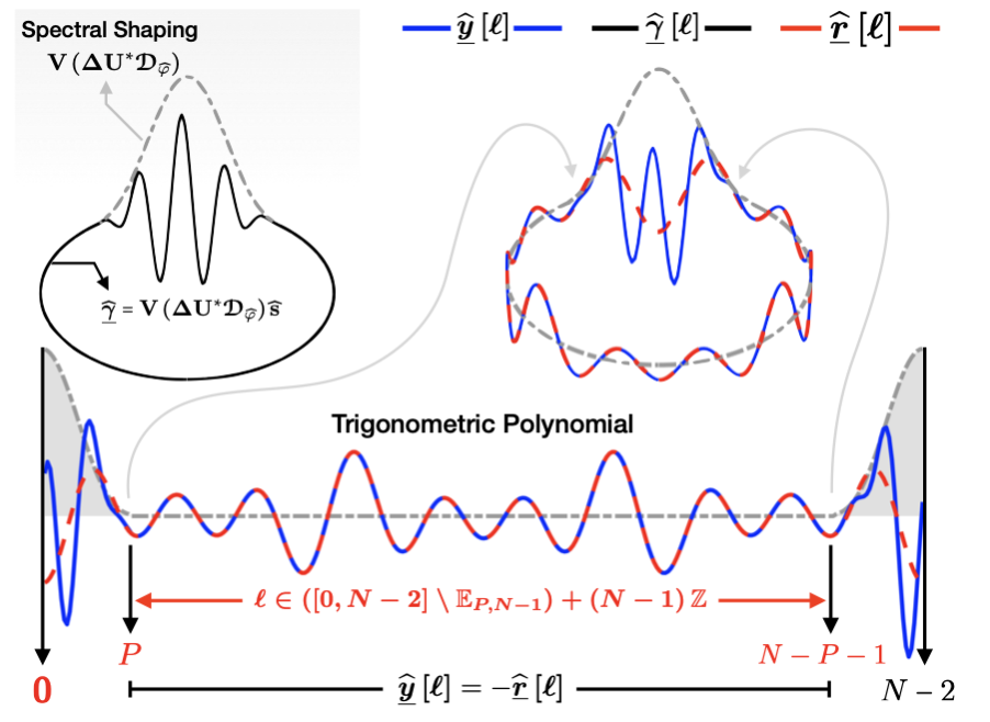
The approach for modulo-based dToF leverages a double-sparsity property of the finite differences modulo samples \(\underline{\mathbf{y}}\). In the Fourier-domain,
The first component in the RHS is the known spectrum shaping filter \(\mathbf{V}\boldsymbol{\Delta}\mathbf{U}^{\ast}\mathcal{D}_{\widehat{\varphi}}\), applied to the sparse signal \(\widehat{s}\).
The residual component \(\underline{\mathbf{r}}\) is sparse with \(2M\) parameters, where \(M\) is the number of folds.
Suppose that we are given \(K\) modulo samples \(y[k] = \mathscr{M}_{\lambda}(g(kT)), T > 0\) folded at most \(M_{\lambda}\) times, where \(g = (s_{N} * \phi)\) and where \(s_{N}(t) = \sum_{n=0}^{N-1} \Gamma_{n} \delta(t - t_{n})\) is an unknown \(N\)-sparse signal and \(\phi \in \mathcal{B}_{\Omega}\), is a known, \(\tau\)-periodic kernel.
Then, a sufficient condition for recovery of \(s_{K}\) from \(\{y[n]\}_{n=0}^{N-1}\) is that
Given the finite-differences sequence, \(\underline{\mathbf{y}}\), the recovery steps are:
Set \(\widehat{\underline{\boldsymbol{\gamma}}}=\mathbf{V}\boldsymbol{\Delta}\mathbf{U}^{\ast}\mathcal{D}_{\widehat{\varphi}}\mathsf{\widehat{s}}\). The \(K\)-length DFT \(\widehat{\underline{\mathbf{y}}}\) can be partitioned as
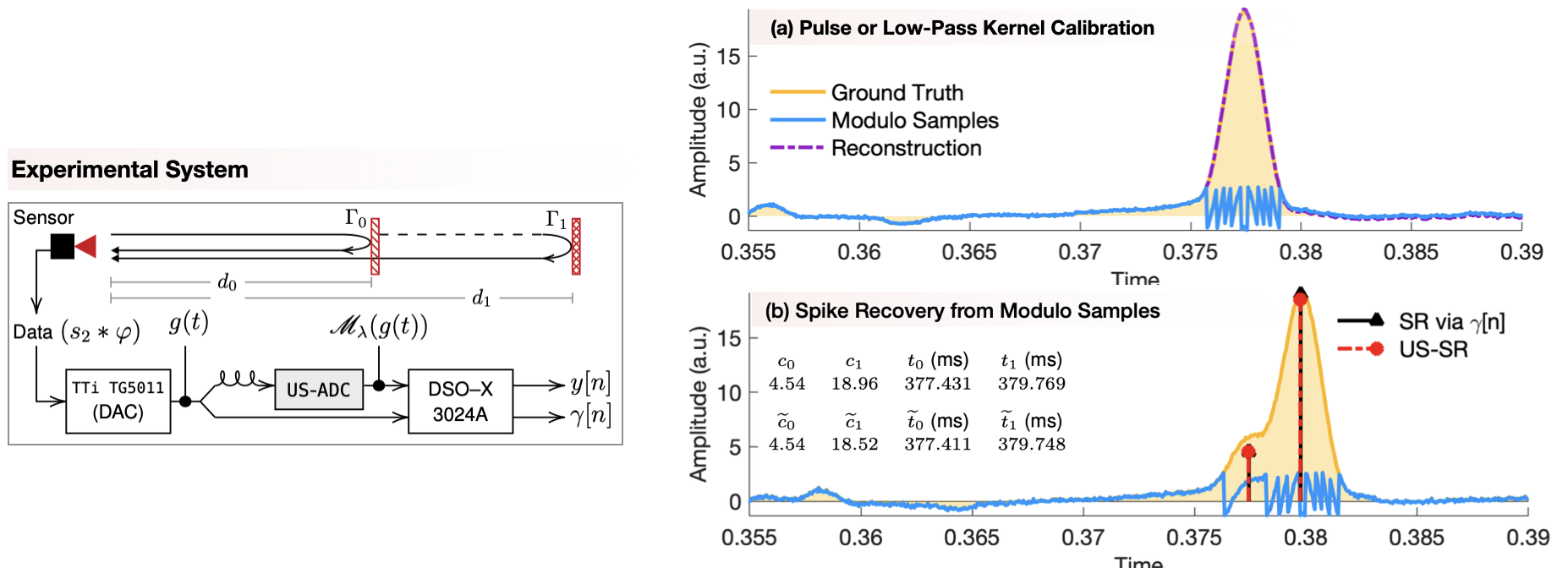
Hardware Experiments
In a hardware experiment, the lowpass projections of a signal containing two distinct reflections where digitized by the M-ADC.
The maximum input signal amplitude was set to \(\approx9.5\lambda\) and the maximum kernel amplitude to \(\approx9.5\lambda\).
Given the modulo samples, the US-SR algorithm was tested, achieving an absolute error in amplitude reconstruction of \(10^{-2}\) and an absolute error in time reconstruction of \(10^{-4}\) seconds.