Conventional ADCs can reliably record signal amplitudes only within a finite dynamic range, and amplitudes outside this range lead to clipping or saturation, causing information loss.
In the Unlimited Sampling Framework, clipping is completely prevented by encoding the signal into a low-dynamic-range, folded representation.
This encoding relies on a non-linear mapping performed by the hardware. Specifically, the input signal amplitudes pass through a modulo operator, \(\mathscr{M}_\lambda\), in the analog domain. This operation, with respect to the threshold \(\lambda\), is mathematically described as:
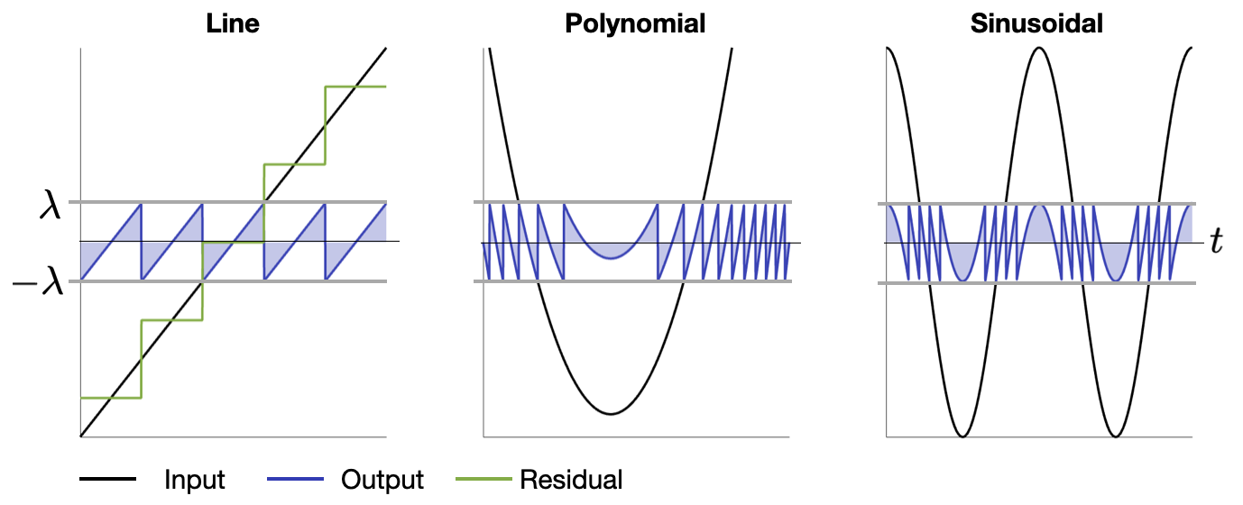
where \([f] = f - \lfloor f \rfloor\) defines the fractional part of \(f\) and \(\lambda > 0\) is the ADC threshold. The following input-output pairs illustrate modulo folding in action.
Fig. 1 Modulo output for different input signals.
Shown in green in the left figure, is the residual part of the modulo operation. This piecewise constant function is in fact the quantized signal that is record by a conventional ADC. In contrast, the modulo signal that is recorded by the M-ADC corresponds to the quantization noise!
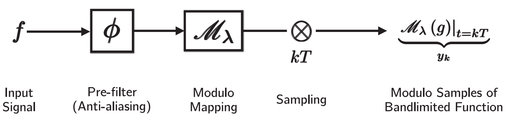
The \(\mathscr{M}-\mathsf{ADC}\) generates the quantization noise signal, which is then sampled and recorded. The acquisition pipeline of the \(\mathscr{M}-\mathsf{ADC}\) is shown in the next figure.
More information on the implementation of the modulo hardware is here.
Fig. 3 Conventional sampling with clipping (a) and modulo sampling (b).
One of the key achievements of the USF is proving that, under certain conditions, the quantization noise is a bounded representation that preserves all information from the original signal. The conditions depend on the input signal class, as further explained in the Signal Classes section.
As this is computational sensing architecture, the modulo-ADC produces encoded samples of the signal to be recovered. Then, a decoding algorithm is needed to extract the desired information from the samples. More information about recovery algorithms is in the Algorithms section.
Conventional wisdom in sampling suggests that dynamic range and noise floor are trade-offs: for a fixed bit budget, increasing dynamic range generally requires larger quantization steps, and vice versa.
Notably, unlimited sampling breaks this notion. While modulo signals effectively encode high input amplitudes, they also allow lower quantization steps, thereby achieving both higher dynamic range and improved resolution simultaneously.
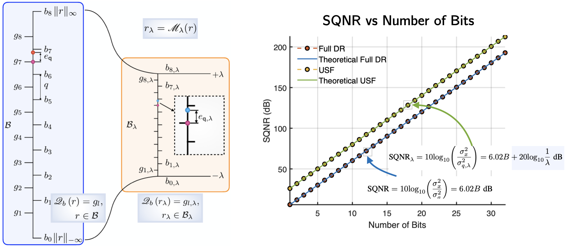
Fig. 4 Left: Illustration of the quantization process for bit resolution b = 3. Right: Comparison between the SQNR of a conventional and the modulo ADCs.
To measure the quality of the quantization, the signal-to-quantization noise is defined by \(\mathsf{SQNR} = 10 \log_{10} \left(\frac{\sigma_{\mathsf{q}}^{2}}{\sigma_{g}^{2}}\right)\), where \(\sigma_{r}^{2}, \sigma_{\mathsf{q}}^{2}\) denote the power of the signal \(g\) (assuming zero mean) and the quantization noise, respectively. For the M-ADC, the quantization error \(\sigma_{\lambda, \mathsf{q}}^{2}\) is decreased due to the modulo operation by a factor of :
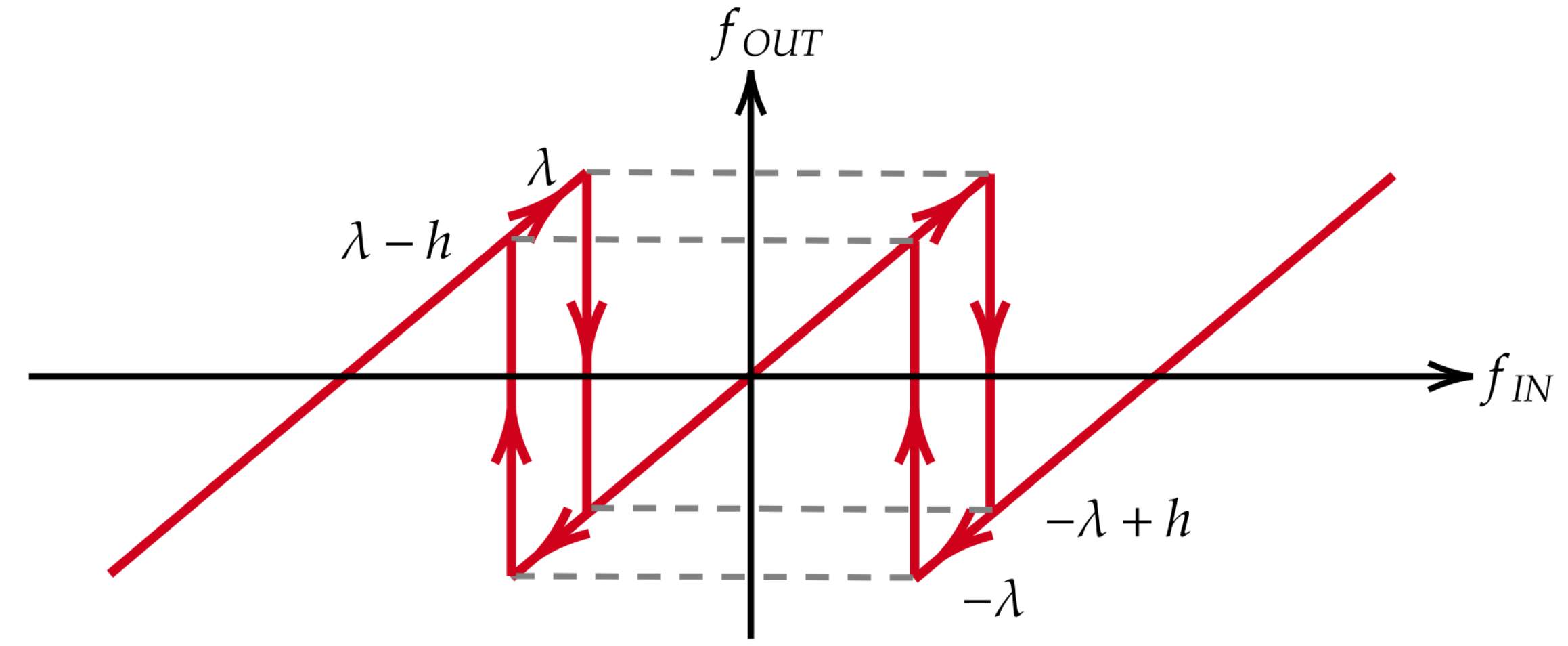
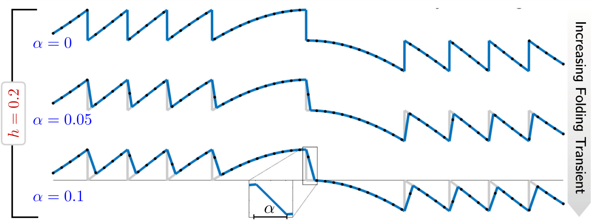
Generalized modulo model was introduced in [6] where two new degrees of freedom were introduced.
a) Hysterisis\(h\) - output of the at a given time depends on the history of the input.
b) Folding Transient\(\alpha\) - physical non-idealities due to slew-rate play a role and hence the exact transitions can not be realized.
Fig. 5 Effect of Folding Transient \(\alpha\) on Generalized Modulo Encoder.
Generalized Modulo Encoder
The analog modulo encoder with encoder threshold \(\lambda\), hysterisis parameter \(h \in [0, 2\lambda)\)
and transient parameter \(\alpha\), is an operator \(\mathscr{M}_\mathsf{H} : \mathsf{PW}_\Omega \rightarrow L^2 ({\mathbb R}), \mathsf{H} = [\lambda, h, \alpha]\),
that generates an asynchronous sequence \(\{ \tau_p \}\) and an analog function \(z(t) = \mathscr{M}_\mathsf{H} g(t), t \geq \tau_0\)
in response to input \(g\). The sequence \(\{ \tau_p \}\) is computed recursively as
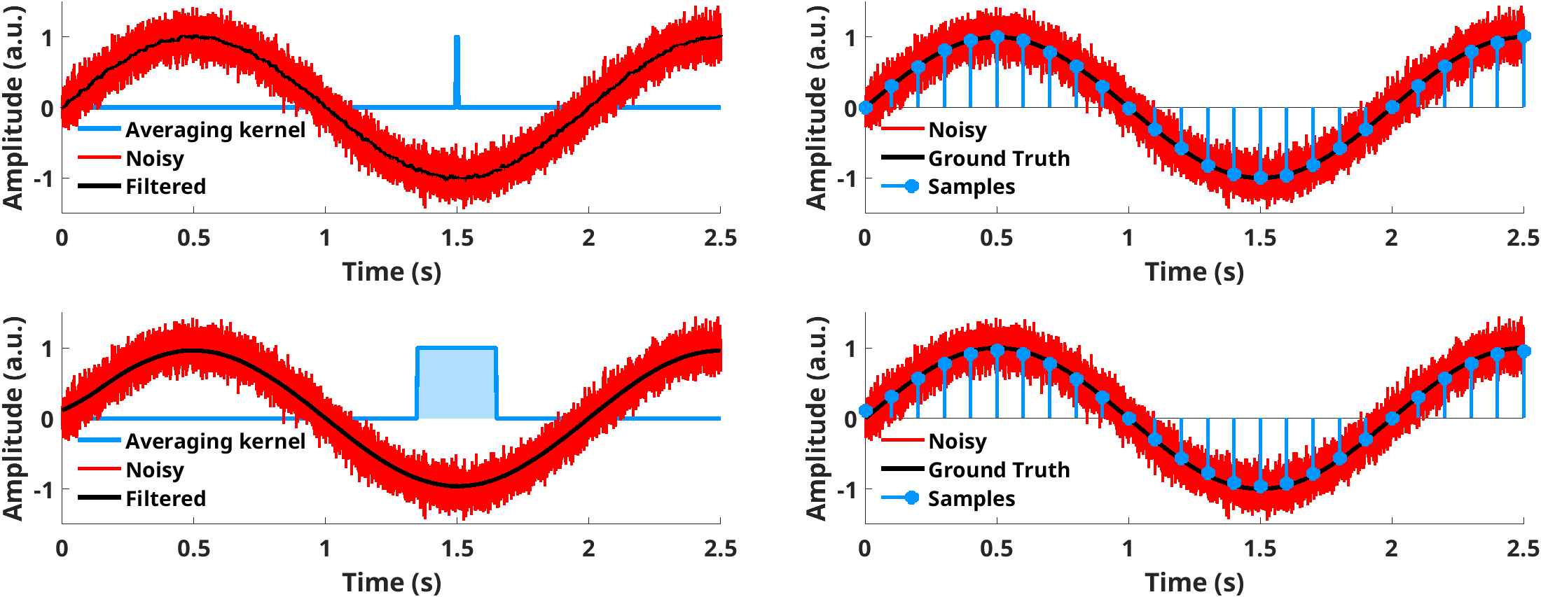
During practical signal acquisition, the sampled value does not have to be exact but instead corresponds to average over neighbouring values.
This effect can be modelled as a convolution of the input signal \(g(t)\) with averaging kernel \(\psi(t)\). The effect of the averaging kernel
on the acquired signal is shown in Fig. 6. The averaging kernel can be also used for denoising
at the cost of resolution.
Hardware experiments have shown that when input signal frequency is much larger than the operational bandwidth of modulo ADC, the samples can be more accurately modelled as local averages than ideal pointwise samples.
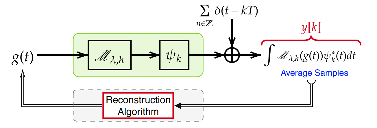
Unlimited Sampling with Local Averages was considered in [7] where we have proposed following acquisition pipeline.
Fig. 7 Unlimited Sampling acquisition pipeline with averaging filter
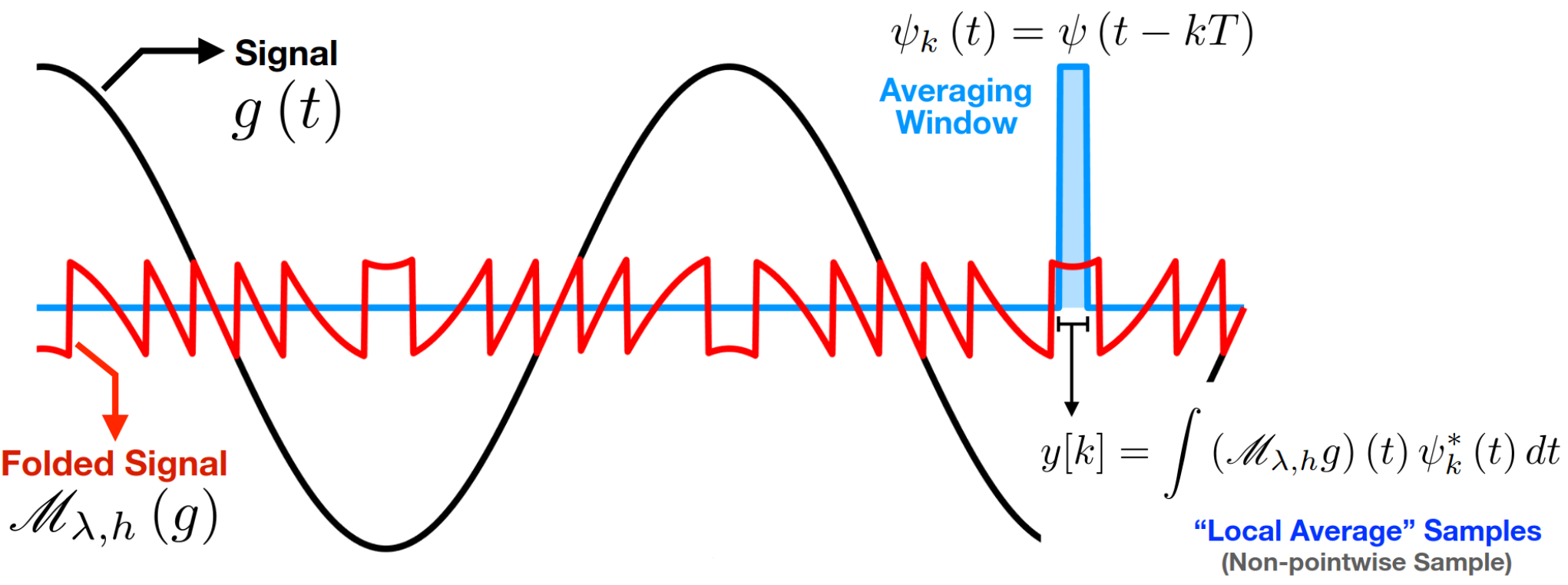
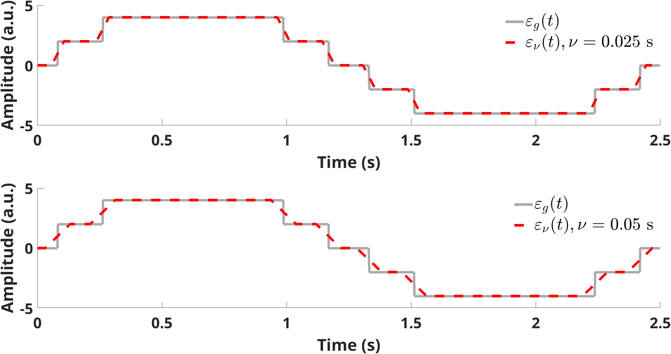
The modulo signal \(\mathscr{M}_{\lambda,h}(g(t))\) filtered with average kernel \(\psi_k(t)\) is visually depicted in Fig. 8.
where \(\epsilon_0(t) = (t + \nu)\frac{\lambda_h}{\nu}{\mathbb I}_{[-\nu, \nu]}(t) + 2 \lambda_h \cdot {\mathbb I}_{[\nu, \infty)}(t)\)
is not a sharp staircase function anymore. \(\epsilon_\nu(t)\) shown in Fig. 9 is a step function with amplitude \(2 \lambda_h\)
and a transient period of duration \(2\nu\) and slope \(\lambda_h / \nu\).
The power consumption of the ADC grows linearly with increasing frequency and exponentially with the number of quantization bits.
Low resolution acquisition architectures make a trade-off by reducing the number of quantization bits and increasing the oversampling
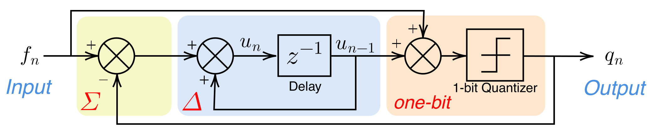
factor. One of the popular one-bit acquisition architecture is \(\Sigma\Delta\) Quantizer described by the following diagram.
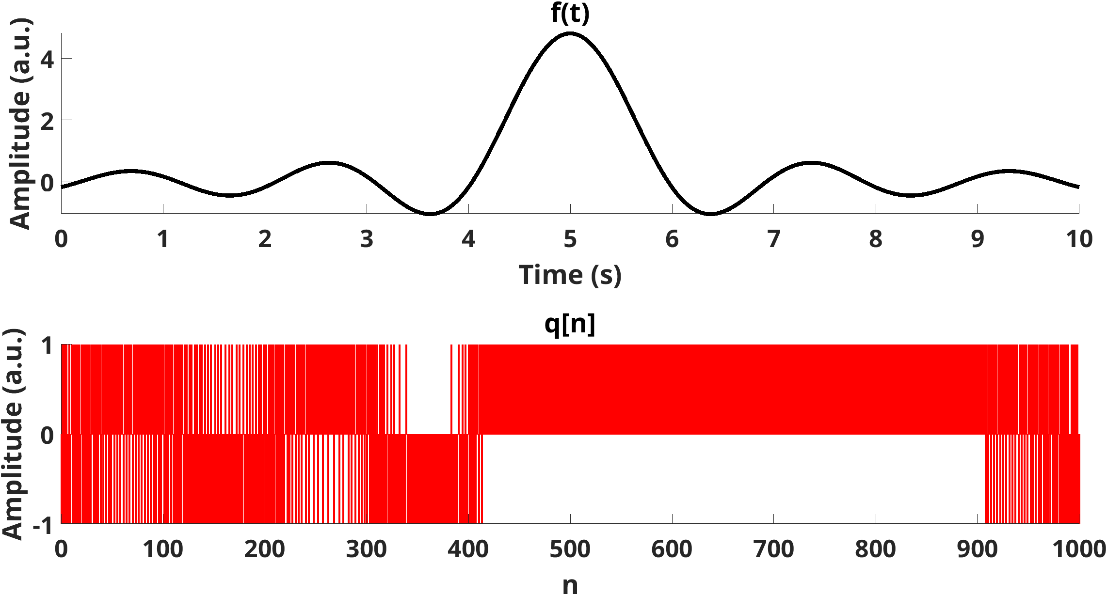
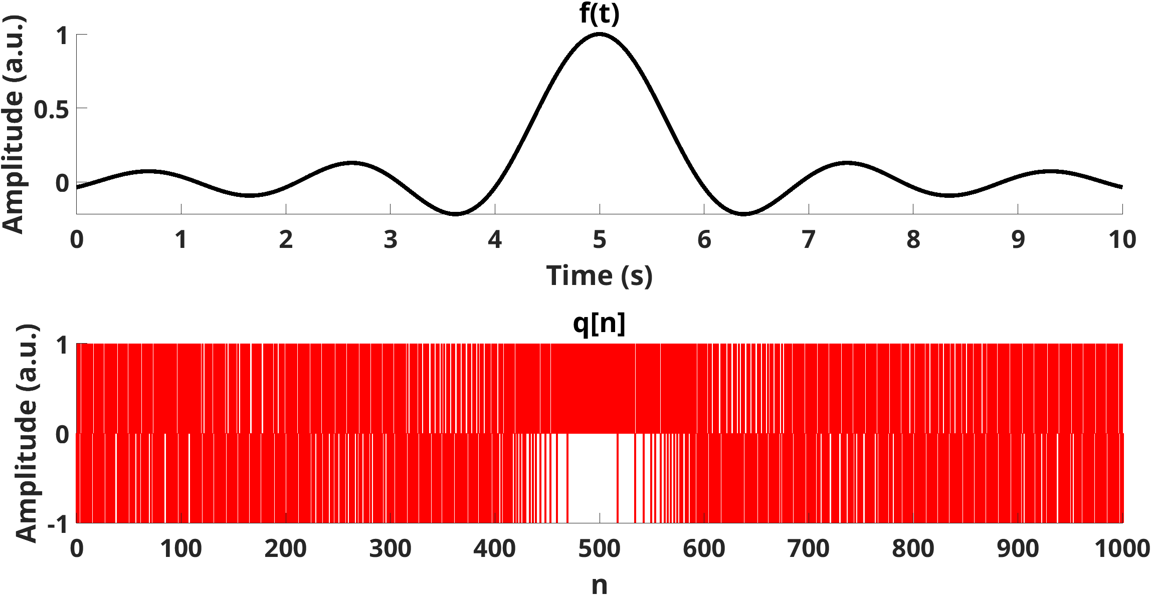
The filter \((1 - z^{-1})\) pushes quantization noise into high frequency regions as it can be seen from the DFT of \(q[n]\)
and the energy of \(f[n]\) is preserved in the bandlimited region.
The key limitation of conventional \(\Sigma\Delta\) is the assumption that input signal is within the DR of the quantizer.
When DR of the input signal \(f(t)\) exceeds the quantizer threshold, signal information is lost as shown in Fig. 13.
Fig. 13 Saturation of \(\Sigma\Delta\) Quantizer.
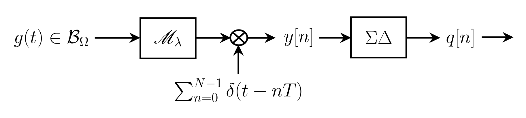
To prevent quantizer saturation, modulo architecture with \(\Sigma\Delta\) quantizer was considered in [8]. The proposed acquisition architecture can be described by the following diagram.
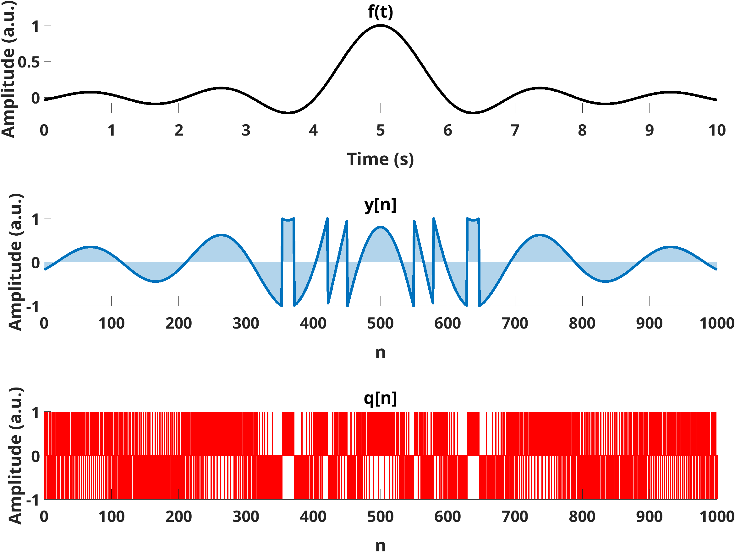
Fig. 14 USF Architecture with \(\Sigma\Delta\) quantizer.
The input-output characteristics together with modulo samples \(y[n]\) is shown in Fig. 15.
Another alternative to conventional pointwise sampling is time-encoding or even-driven sampling. This strategy involves
discretizing time axis instead of discretizing amplitude. One of the approaches to implement time-encoding is asynchronous
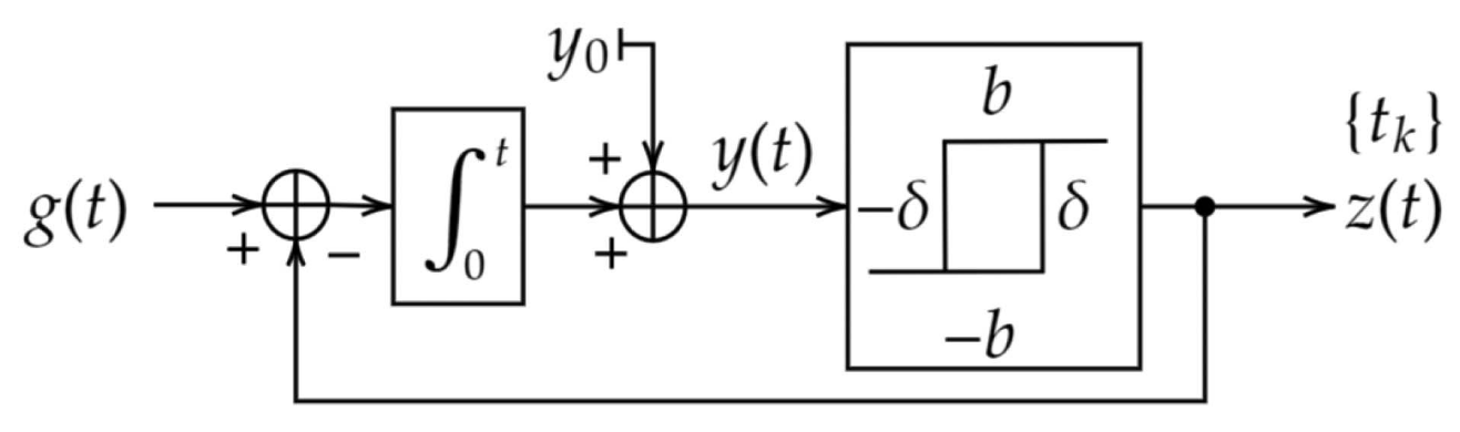
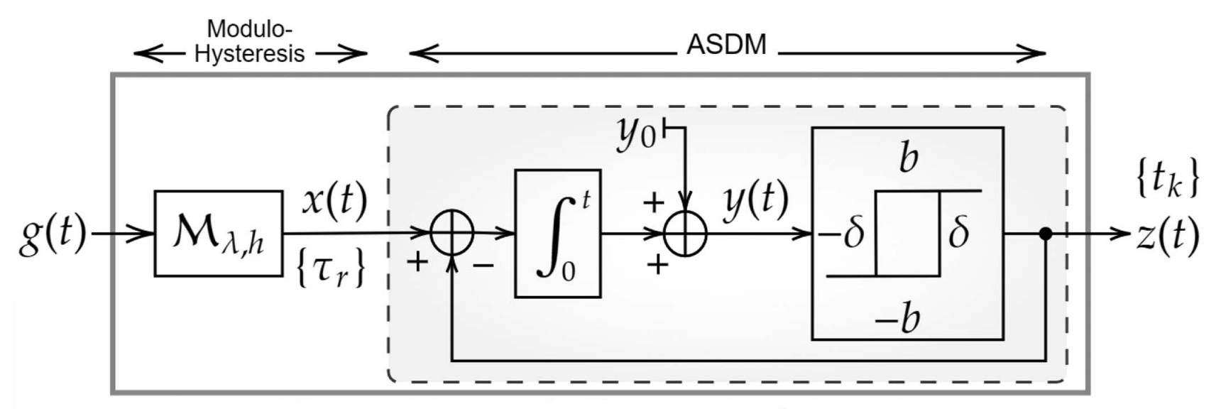
sigma-delta modulator (ASDM) depicted in Fig. 16. ASDM ads input \(g(t)\) to the current state
\(z(t)\), which is then processed with an integrator with initial condition \(y_0\) followed by a Schmitt trigger
with parameters \(\delta, b\).
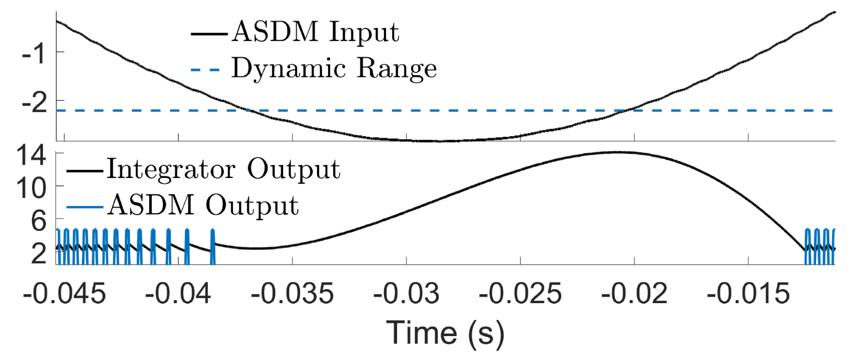
When \(||g(t)||_\infty\) exceeds \(b\), a recovery from ASDM measurements is no longer possible
since the dynamic range of the ADC is exceeded. This scenario is depicted in Fig. 17.
Fig. 17 Saturated output of a conventional ASDM with \(\delta = 1\) and \(b = 1\).
To solve the saturation issue in conventional ASDM, Modulo-Hysterisis Event-Driven Sampler (MEDS) was proposed in [9]. The designed acquisition sampling architecture is depicted in depicted in Fig. 18.
In analogy to Shannon’s sampling theorem, our first result [10], the Unlimited Sampling Theorem proves that a bandlimited signal can be recovered from modulo samples provided that a certain sampling density criterion, that is independent of the ADC threshold, is satisfied. In this way, our result allows for perfect recovery of a bandlimited function whose amplitude exceeds the ADC threshold by orders of magnitude.
Let \(f(t)\) be a function with no frequencies higher than \(\Omega\) (rad/s), then a sufficient condition for recovery of \(f(t)\) from its modulo samples \(y_{k} = \mathscr{M}_{\lambda}(f(t_{k}))\) taken on grid \(t = k T_{\epsilon}, \ k \in \mathbb{Z}\) is,
\[T \leq \frac{1}{2\Omega e}.\]
Uniqueness Conditions
In fact, there is a one-to-one mapping between a bandlimited function and its modulo samples provides that the sampling rate is higher than the critical rate of the Nyquist rate, \(T<\pi / \Omega\). The Injectivity Conditions are proved in [2].
Injectivity
Let \(f(t)\) be a finite-energy function with no frequencies higher than \(\Omega\) (rad/s). Then the function \(f(t)\) is uniquely determined by its modulo samples \(y_{k} = \mathscr{M}_{\lambda}(f(t_{k}))\) taken on grid \(t = k T_{\epsilon}, \ k \in \mathbb{Z}\), where
When working with bounded noise, we assume that the modulo samples \(y[k]\) are affected by noise \(\eta\) of amplitude bounded by a constant \(b_{0} > 0\). That is,
\[\forall k \in \mathbb{Z}, \quad y_{\eta}[k]= y[k] + \eta\left[ k \right], \quad \left| {\eta \left[ k \right]} \right| \leqslant b_0.\]
Note that due the presence of noise, it may happen that \(y_{\eta}[k] \not\in [-\lambda,\lambda]\). Nonetheless, for \(b_{0}\) below some fixed threshold, our recovery method provably recovers noisy bandlimited samples \(\gamma[k]\) from the associated noisy modulo samples \(y_{\eta}[k]\) up to an unknown additive constant, where the noise appearing in the recovered samples is in entry-wise agreement with the one affecting the modulo samples. That is, \(\widetilde \gamma \left[ k \right] = \gamma \left[ k \right] + \eta \left[ k \right] + 2m\lambda, m\in \mathbb{Z}\).
Let \(g(t)\) be an \(\Omega\)-bandlimited and finite-energy signal. Assume that \(\beta_{g} \in 2\lambda \mathbb{Z}\) is known with \(||g||_\infty\leqslant \beta_{g}\). For the dynamic range we work with the normalization \(\mathsf{DR} = {\beta_{g}}/{\lambda}\). Let the noisy modulo samples with a noise bound given in terms of the dynamic range as,
Then a sufficient condition for the approximate recovery of the bandlimited samples \(\gamma[k]\) is that,
\[T \leq \frac{1}{2^{\alpha}\Omega e}.\]
The recovery is approximate in the sense that, \(\widetilde \gamma \left[ k \right] = \gamma \left[ k \right] + \eta \left[ k \right] + 2m\lambda, m\in \mathbb{Z}\).
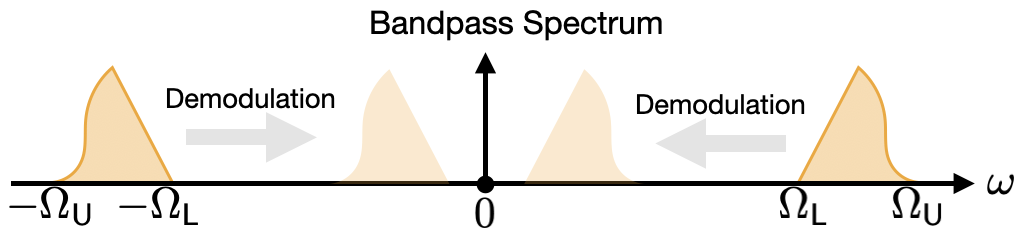
Bandpass signals form a sub-class of bandlimited signals that arise in various applications including sonar, radar, ultrasound and RF communications. A mathematical model for this class is,
Due to their high-frequency content, acquisition based on Shannon’s sampling theorem is challenging in practice, and necessitates the development of techniques to overcome this.
One such technique is bandpass sampling, where carefully chosen sub-Nyquist sampling rates are used.
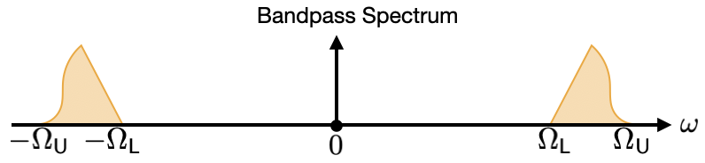
The Fourier structure of bandpass signals implies that for some rates, the spectral information is translated into the sampled spectrum without overlaps. These rates are illustrated in the next figure.
Bandpass and Unlimited Sampling. Bandpass sampling and the USF address distinct ADC limitations (conversion speed, dynamic range and resolution), however in practice they may co-exist.
To implement Unlimited bandpass sampling, which is a solution that simultaneously addresses all the limitations, integration of two significantly different techniques is required:
In bandpass sampling, undersampling compresses the spectral information into a smaller frequency range.
In unlimited sampling, the modulo operation transforms a bandlimited input into a non-bandlimited signal. Recovery is made possible through oversampling.
Figure of bandpass spectrum and modulo spectrum
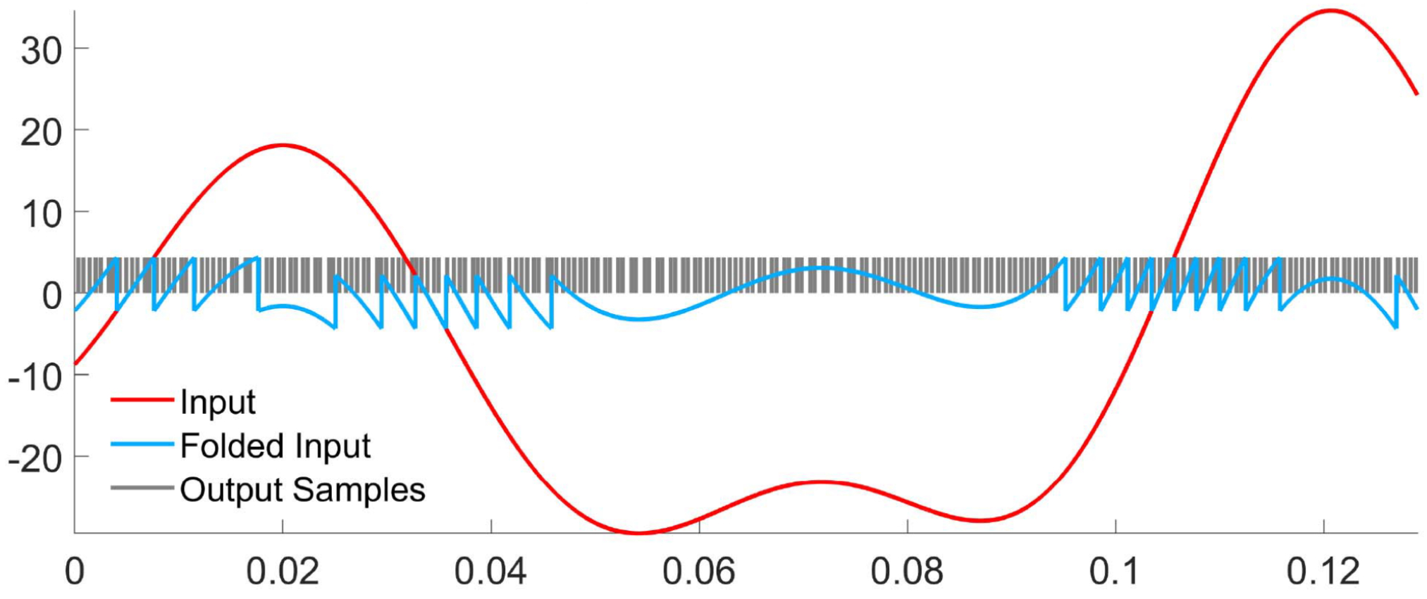
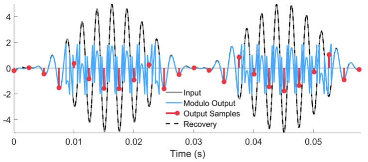
How modulo signals are affected by undersampling? Using undersampling rates to reconstruct a bandpass signal from its modulo samples may seem counterintuitive, but the following figure offers some insight.
The hardware experiment shows modulo samples of a bandlimited signal (in red) observed at an undersampling rate \(\Omega_{\mathsf{S}}\), alongside the corresponding bandpass signal.
Interestingly, the modulo and bandpass samples align, suggesting that although modulo signals spread energy across the spectrum, the bandpass information remains localized and can be reconstructed by adjusting sampling rates.
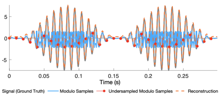
To formalize the above, we let \(g[k]\) represent the samples of a bandlimited signal \(g(t)\), that are generated by applying a lowpass filter with bandwidth s to the samples of a bandpass signal \(g_\mathsf{BP}(t)\).
Then, the modulo undersampling principle is that whenever \(g_{\mathsf{BP}}[k]=g[k]\), then \(y_{\mathsf{BP}}[k]=y[k]\).
Unlimited Sampling of Bandpass Signals. The bandwidth of \(g(t)\) comes from the mapping of the spectra of \(g_BP(t)\) to \(g(t)\), and depends non-linearly on the sampling rate \(\Omega_{\mathsf{S}}\).
However, it can be solved to guarantee a sufficient oversampling of \(g(t)\) that would allow its recovery from the modulo samples \(y_\mathsf{BP}[k]\). For the recovery of \(g_{\mathsf{BP}}\), valid sampling rates must also guarantee
one-to-one mapping between the spectra of \(g_{\mathsf{BP}}\) and \(g\). The result is summarized in the following theorem.
Let \(g_{\mathsf{BP}}(t)\) be a bandpass signal and \(z_{\mathsf{BP}}(t)=\mathscr{M}_{\lambda}(g_{\mathsf{BP}}(t))\). Let \(y_{\mathsf{BP}}[k] = z(k T_{\mathsf{s}})\), \(k \in \mathbb{Z}\) be the modulo samples of \(g_{\mathsf{BP}}(t)\) at period \(T_{\mathsf{s}} > 0\). If there exists \(P \in \mathbb{N}\) such that \(T_{\mathsf{s}}\) satisfies,
This result demonstrates that bandpass signals can be perfectly recovered from their modulo samples without oversampling, achieving sub-Nyquist USF.
To observe the effect of undersampling on the spectrum of modulo and bandpass signals and the recovery algorithm:
Online Python Playground USF-BP
For practical modulo bandpass sampling in non-ideal and modulo-hysteresis architectures, a similar rationale can help derive feasible sampling rates. Since these architectures are implemented in hardware, validation on real data is possible.
Given a set of \(K\) discrete samples, \(\{g_{k}\}_{k=0}^{K-1}, \ g_{k}=g(kT)\), the unknown parameters \(\{c_{p}, \omega_{p}\}_{p=0}^{P-1}\) can be estimated from \(K \geq 2P\) measurements using, for example, Prony’s method.
When modulo samples \(\{y_{k}\}_{k=0}^{K-1}\) are observed, it is possible to unfold \(2P\) consequent samples of \(g_{k}\) from \(\{y_{k}\}_{k=0}^{K-1}\) based on the local reconstruction conditions given in CITE. Then, one can use \(\{g_{k}\}_{k=0}^{2P-1}\) for the parameter estimation. The result is summarized by the following theorem.
Unlimited Sampling of Sparse Sinusoidal Mixture [3]
Let \(g \in \mathcal{B}_{\pi}\) be the \(P\)-sparse sinusoidal mixture to be recovered, and assume that \(\beta_{g} \geq ||\mathbf{c} ||_{\ell_{1}}\) is known. Let \(y_{k} = \mathcal{M}_{\lambda} (g (t))|_{t=kT} , k = 0, . . . , K − 1\) be the modulo samples of \(y(t)\) with sampling rate \(T\). Then a sufficient condition for recovery of \(g(t)\) from \(y_{k}\) (up to additive multiples of \(2\lambda\)) is that
Sparse signal recovery from low-pass filtered samples is an important topic related to the research topics of Tauberian approximation, super-resolution, sparse deconvolution, and finite-rate-of-innovation sampling. It also finds applications in time-resolved imaging. Given a \(P\)-sparse signal to be super-resolved as,
where \(\varphi\) is a known, bandlimited and \(\tau\)-periodic kernel, \(\bar{\varphi}(t)=\varphi(-t)\). The goal is to recover \(s_{P}\) from its modulo samples, that is \(y_{k} = \mathcal{M}_{\lambda} (g (t))|_{t=kT} , k = 0, . . . , K − 1\).
Let \(g = s_{P}\ast \varphi\), where \(s_{P}\) is an unknown \(P\)-sparse signal and \(\varphi\) is a known bandlimited, \(\tau\)-periodic kernel. Let \(\{y_{k}\}_{k=0}^{K-1}\) be \(K\) modulo samples of \(g(t)\) with sampling rate \(T\), folded at most \(M_{\lambda}\) times. Then a sufficient condition for recovery of \(s_{K}\) from \(\{y_{k}\}_{k=0}^{K-1}\) (up to additive multiples of \(2\lambda\)) is that
![DFT of :math:`q[n]`.](_images/qn_dft.png)