Modulo samples encode the original input signal, and extracting this information requires an algorithmic decoding process. A variety of recovery algorithms have been developed, tailored to the specific sampling architecture and desired output—whether full signal reconstruction (unfolding) or extraction of certain parameters.
In most of the existing algorithm, the modulo decomposition property is leveraged.
Modular Decomposition Property
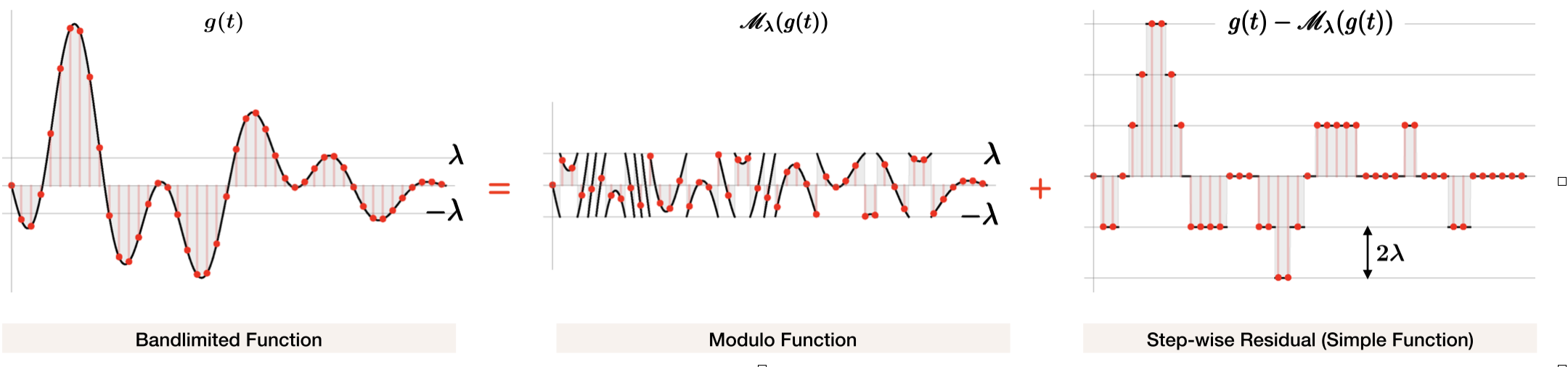
Let \(g \in \mathcal{B}_\Omega\) and \(\lambda\) is a fixed, positive constant. Then, the bandlimited function
\(g(t)\) admits a decomposition
where \(\varepsilon_g\) is a simple function, referred to as the residual.
Notice that if the modulo part of a signal is known, then knowing its residual \(\varepsilon\) is equivalent to knowing \(g\). However, the fact that the residual has a piecewise constant structure can be used as a prior for its recovery.
This algorithm is the first one to appear for decoding of modulo samples produced by the ideal \(\mathscr{M}-\mathsf{ADC}\) architecture (so \(\varepsilon(t) \in 2\lambda{\mathbb{Z}}, \forall t\)). It was presented in [10], [1] and is guaranteed to recover a bandlimited signal from its modulo samples if the sampling rate satisfies the Unlimited Sensing Theorem.
Notably, the sampling rate does not depend of the modulo threshold.
The algorithmic procedure leverages the properties of the two signals that decompose the modulo signal:
The smoothness of the bandlimited signal is used to separate it from the residual in the higher-order-differences space.
The restriction of the residual amplitudes to the range \(2\lambda{\mathbb Z}\) is used to find the constants of integration, and to form a stable inversion process.
The key algorithmic steps are described below. For the full details: [10], [1].
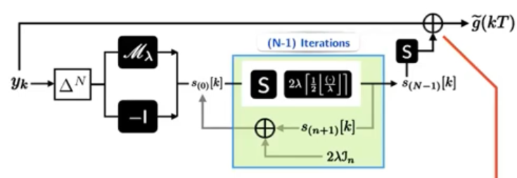
US-Alg
Compute \(\Delta^{N}y\), the \(N^{\mathrm{th}}\) order finite differences of the modulo sequence \(y[k]\).
Apply \(\mathscr{M}_{\lambda}(\Delta^{N}y)\). | Since \(\mathscr{M}_{\lambda}(\Delta^{N}\epsilon)=0\), we get \(\mathscr{M}_{\lambda}(\Delta^{N}y) = \mathscr{M}_{\lambda}(\Delta^{N}g)\). For sampling rates that satisfy the Unlimited Sensing Theorem, that is \(T \leq 1 / (\Omega e)\), the maximal amplitude of the sequence \(g[k]\) shrink with the finite-differences order such that \(||\Delta^{N}g||_{\infty} \leq (T \Omega e)^{N}||g||_{\infty}\), where \(||\cdot||_{\infty}\) denotes the max-norm. If .. math:: N = leftlceil frac{log lambda - log beta_g}{log (T Omega e)} rightrceil , quad beta_g in 2lambda mathbb{Z} text{ and } beta_g geq | g |_infty, | then \(\| \Delta^{N}g \|_{\infty} \leq \lambda\). This implies \(\mathscr{M}_{\lambda}(\Delta^{N}y) = \Delta^{N}g\).
Compute \(\Delta^{N}r[k] = \mathscr{M}_{\lambda}(\Delta^{N}y) - \Delta^{N}y\), the \(N^{\mathrm{th}}\) order finite differences of the residual sequence \(r[k] = \epsilon(kT)\).
Set \(s_{(0)}[k] = \left( \Delta^{N}r \right)[k]\). | For \(n = 0 : N - 2\):
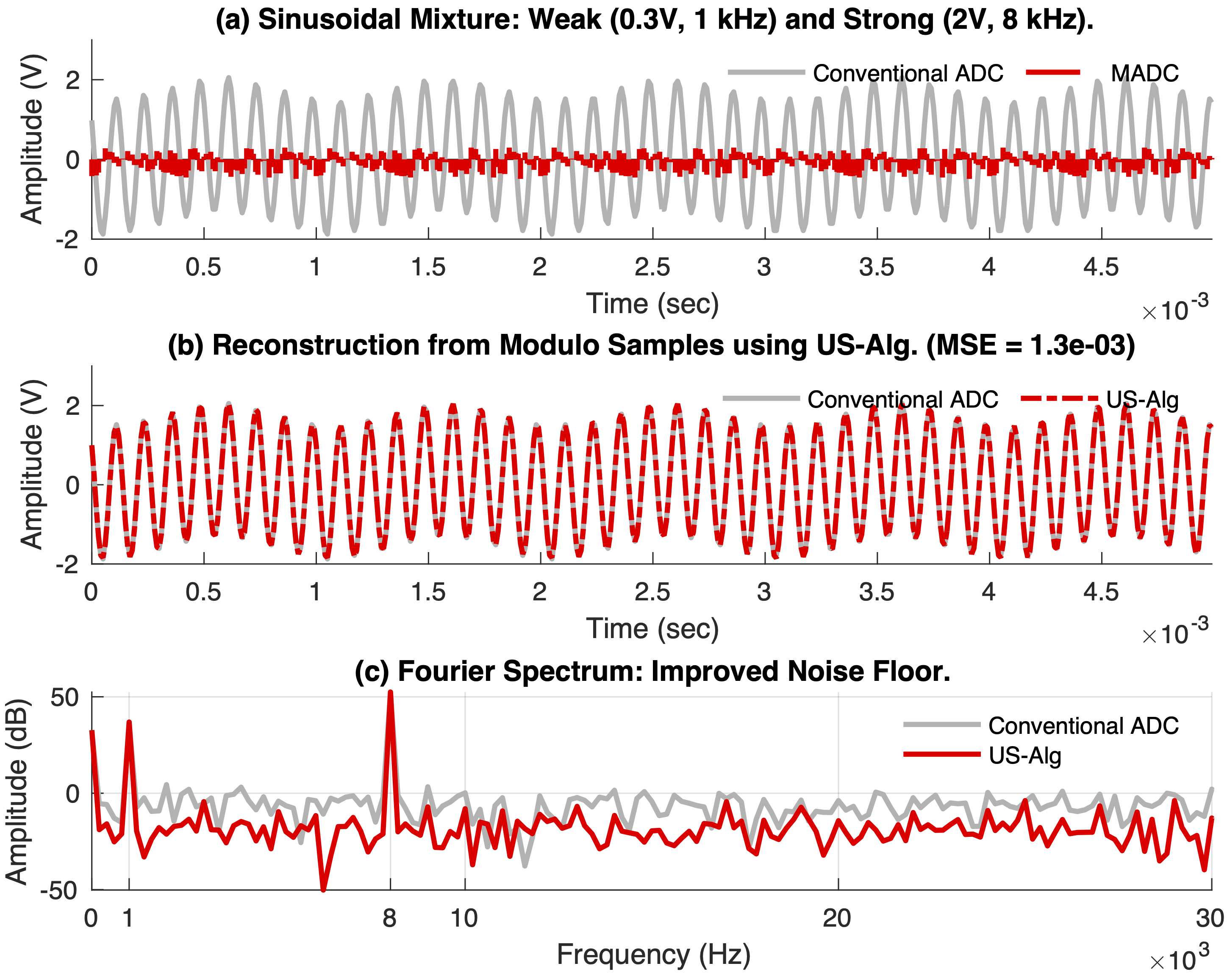
The input \(g\) consists of a sinusoidal mixture: weak component with \(0.3\) V at \(1\) kHz, and a strong component with \(2\) V at \(8\) kHz. The modulo ADC (MADC) based on [1], [6], [11], [12] is deployed with \(5.40\)-folds dynamic range extension, sampling rate of \(100\) kHz and quantization resolution of \(6.7\)-bit.
In this scenario, the MADC measurements (\(500\) samples) entails intensive modulo-folds (degrees-of-freedom of \(\varepsilon\)\(=330\)). Despite these challenging settings, we use the US-ALG for reconstruction with fourth-order difference or \(N=4\), achieving an signal recovery with a mean-squared error \(\propto 10^{-3}\).
Fig. 22 Hardware Validation: Signal Reconstruction using US-ALG with Fourth-order difference.
The key idea in reconstructing of the original samples from measurements encoding via \(\mathscr{M}_\mathsf{H}\) is to convolve modulo samples \(y[n]\) with a filter \(\psi_N[k] \triangleq \Delta^N[k + 1]\) and identify the residual by thresholding.
Assume that \({\psi_N \ast \gamma}_l^\infty < \lambda_h / (2N)\) and let \(k_m, k_m \in \mathbb{Z}\) defined as in (11).
Furthermore, let \(\tilde{n}_1\) and \(\tilde{s}_1\) be the estimations of the discrete folding time and sign defined as
Folding parameters \(\tilde{\tau}_p\) and \(\tilde{s}_p\) can be sequentially computed with previous Theorem sequentially, if the supports of each of two filtered folds are disjoint.
This requires the separation of the folding times \(n_{p+1} - n_p \geq N + 1\), which is guaranteed if
\[\frac{h^*}{T\Omega g_\infty} \geq N + 1\]
Denote \(p\) as index for folding index and let \(\mathcal{K}_N = \bigcup_{p \in [1, P]} \left\{ k_m^p, k_M^p \right\}\), where the pairs \(\left \{ k_m^p, k_M^p \right \}\) are computed sequentially as follows. For \(p = 1\)
To estimate \(e[k]\) from \(y[k]\) we assume a smoothness property on \(g(t_k)\), i.e. \(||\Delta^N g(t_k) ||_\infty < \frac{\lambda_h}{2 N}\).
Far away from the jump, this condition will also hold for \(y[k]\)
Estimation of Folding Times.
Assume \(||\Delta g(t_k)||_\infty < \lambda_h / 2N\) and let \(k_m = \mathsf{min} {\mathbb M}_N\). Furthermore,
let \(\tilde{\tau}_1 = \tilde{n}_1 T - 2 \nu \beta_1 + \nu\) and \(\tilde{s}_1 = -\mathsf{sign}(\Delta^N y[k_m])\)
be the estimates of the folding time with \(\tilde{n}_1 = k_m + N\) and \(\tilde{\beta}_1\) given by
Input Reconstruction. Input signal is recovered from \(\mathcal{L} \tilde{g}[k] = 2\nu \left ( y[k] + \tilde{\varepsilon}[kT] \right )\),
where \(\mathcal{L} \tilde{g}[k] \triangleq \int_{kT - \nu}^{kT + \nu} \tilde{g}(s) ds\) are the local averages and
Compute \(\left ( \Delta \ast \psi_h^N \right )[n]\) with smoothing kernel \(\psi^N(t) := B^N \left ( \frac{N}{2} t \right ) / \mathsf{max} \left ( B^N (t) \right )\), where \(B^N\) is a B-spline of order \(N\).
Compute \(\mathscr{M}_\lambda\left ( ( \Delta q \ast \psi_h^N ) [n] \right ) - \left ( \Delta q \ast \psi_h^N \right )[n]\) and retain non-zero points to get \(\Delta\tilde{\varepsilon}_g[n]\).
Add \(0\) at the beginning of \(\Delta\tilde{\varepsilon}_g[n]\) and apply summation operator \(\tilde{\varepsilon}_g[n] = \sum_{k = 0}^{n} \Delta \tilde{\varepsilon}_g[k]\).
Signal Model. Consider \(g \in \mathcal{B}_\Omega\) such that \(g(t) = g(t + \tau), \forall t \in {\mathbb R}\):
\[g(t) = \sum\nolimits_{\left | p \right | \leq P} \hat{g}[p] e^{\jmath p \omega_0 t},\quad\omega_0 = \frac{2 \pi}{\tau},\quad P = \frac{\Omega}{\omega_0}\]
where \(\hat{g}[p]\) denotes the Fourier series coefficients such that \(\hat{g}[-p] = \hat{g}^*[p]\) with \(\sum\nolimits_{p}{\left | \hat{g}[p] \right |} ^2 < \infty\).
Signal \(g(t)\) is then inputted into modulo ADC, sampled with a period \(T\) and giving \(y[n] = \mathscr{M}_{\lambda}(g(t))\).
Problem Formulation. Given modulo samples \(y[n]\), number of folds \(K\) and bandwidth \(\Omega\), reconstruct \(g[n]\).
This can be visually depicted by the following figure.
Unknown residue parameters \(\{ c_m, n_m \}_{m = 0}^{M-1}\) can be estimated using Prony’s method from out of the band part of the spectra.
Let \(H(z) = \sum\nolimits_{n=0}^M h[n]z^{-n} = \prod_{m=0}^{M-1} \left ( 1 - u_m z^{-1} \right )\) where \(u_m = \exp(-\jmath \frac{2 \pi n_m}{N - 1})\).
Convolving out band part of spectra \(\hat{\underline{y}}[n]\) with filter coefficients \(\mathbf{h}\) annihilates the sequence for \(l = [K+P, N - P - 1]\) such that
After finding the roots \(u_m\) unknown folding amplitudes can be found using least-squares method. Given residue
parameters \(\{ c_m, n_m \}_{m=0}^{M-1}\) then residue reconstruction \(\underline{\tilde{r}}{n}\) can be obtain from the definition
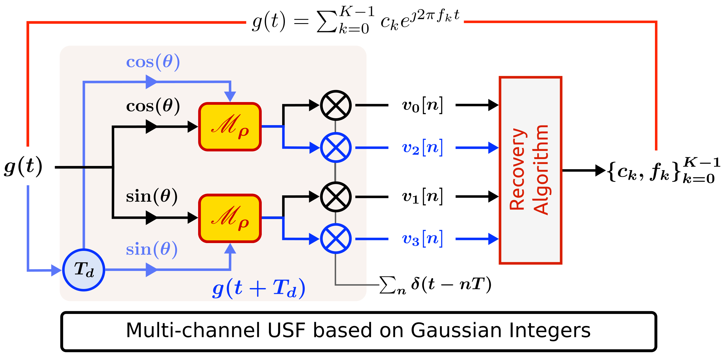
Sub-Nyquist Frequency estimation via USF and the effect of quantization was studied in [14]. Two
multi-channel architectures with modulo acquisition were proposed which enabled the capture of signals \(72\) times exceeding
ADC’s range while achieving \(30000\) times in Nyquist rate reduction.
where signal parameters \(\{ f_k, c_k \}_{k=0}^{K-1}\) are unknown. \(g(t)\) is acquired using the multi-channel
architecture depicted in Fig. 23 which implements thresholds based on Gaussian Integers.
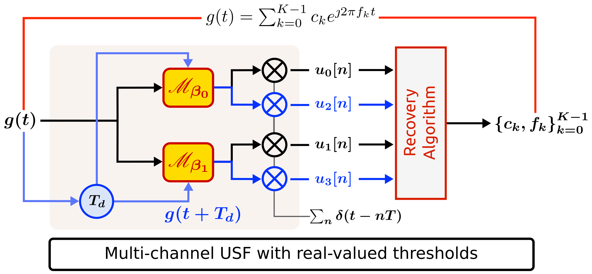
Measurements. Low dynamic range measurements captured by the designed architecture can be described as
Given measurements \(\{ u_l[n] \}_{l=0}^{3}\) captured by the architecture in Fig. 24 with thresholds \(\beta_0\) and \(\beta_1\). Then, \(g(t)\) can be exactly recovered with \(N_{i} \geqslant \left ( 2 - \lfloor \frac{i}{2} \rfloor \right ) K, i\in \mathbb{I}_{4}\) samples provided that \(T_d \leqslant \frac{\pi}{\mathsf{max}_k |\omega_k|}\) and \(\left\| g(t) \right |_{\infty} < \epsilon \frac{\mathsf{c_0, c_1}}{2}\).
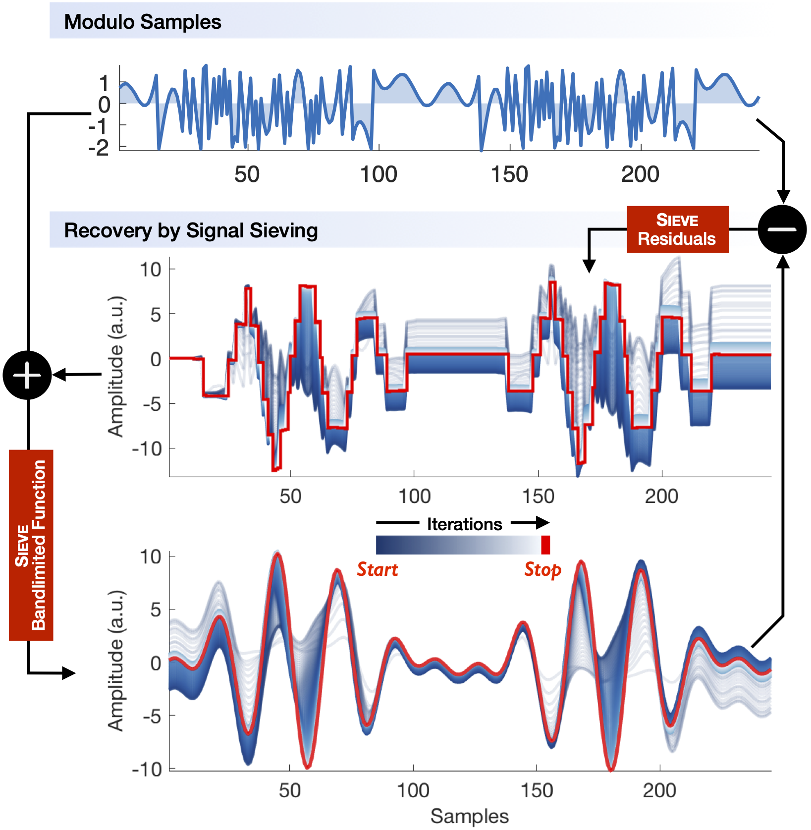
Iter-SiS (Iterative Signal Sieving) is a robust recovery method that operates in the canonical domain [5]. Its core idea is to separate the distinct signal components within the folded samples using an alternating minimization strategy.
where \(T\) denotes the sampling period. \(w\) is the measurement noise characterized by \(\frac{1}{N}\sum\nolimits_{n=0}^{N-1} \left| w\left[n\right] \right|^{2} = \sigma^{2}\).
Here, we specify the noise power rather than assuming a specific stochastic noise distrubution. Our goal is to reconstruct \(\{g[n]\}_{n=0}^{N-1}\) from \(\{y_{w}[n]\}_{n=0}^{N-1}\).
where \(u[\cdot]\) denotes the discrete unit step function. \(c_m\in 2\lambda\mathbb{Z}\) and \(n_{m} \in \mathbb{I}_{N}\) represent the folding threshold and instant, respectively. Denote by :math:’underline{y}[n]=y[n+1]-y[n]’ the finite difference of \(y[n]\). Then, taking the finite difference of (15) leads to,
where \(\underline{\varepsilon}_{g}[n] = \sum_{m=0}^{M-1} c_m \delta[n - n_{m}]\) and \(\delta[\cdot]\) is the discrete delta function.
Hence, the measurements \(y[n]\) can be decomposed as two constituent components: (1) bandlimited signal \(\underline{g}[n]\) and (2) sparse signal \(\underline{\varepsilon}_{g}[n]\). The distinction in signal structures facilitates the separation of the residue \(\underline{\varepsilon}_{g}[n]\), leading to the concept of a signal sieving strategy.
Energy Concentration. Within the finite observation window, \(\underline{g}[n]\) is characterized by enforcing energy concentration in the low-pass region, which is implemented as
Sparse Characterization on the Continuum. To achieve accurate spike estimation, we utilize a continuous-time, parametric representation of the residue,
━━● \(\mathsf{P}(\xi_{N-1}^{n})\) and \(\mathsf{Q}(\xi_{N-1}^{n})\) are trignometric polynomials of degree \(M-1\) and \(M\), respectively with \(\xi_{N-1}^{n} = e^{\jmath \frac{2\pi n}{N - 1}}\).
Hence, in the presence of noise, the signal recovery problem can be formulated as,
where \(\left\lfloor \cdot \right\rfloor\) is the floor function.
To solve (20), we adopt an iterative strategy, namely we construct a collection of estiamtes for \(\mathsf{Q}\) and select the one that minimizes the mean-square error (MSE) in (20). These estimates are found iteratively by solving the minimization below (assuming \(\mathsf{Q}^{[j]} \approx \mathsf{Q}\))
Stopping Criterion. We update the estimates \(\{{\underline{\varepsilon}}_{g}^{[i]}[n], \underline{g}_{\Omega}^{[i]}\}, i\in\mathbb{I}_{i_{\max}}\) through iterating between (21) and (22), until the following criterion is satisfied
This shows that the signal estimates match the original folded measurements within the given tolerance level \(\sigma\). The figure below describes the visual output of the signal sieving process.
Fig. 25 Flowchart of the iterative signal sieving.
The procedure is summarized below:
Iterative Signal Sieving Algorithm
Input.\(\{y_{w}[n]\}_{n=0}^{N-1}, \lambda\) and \(\Omega\).
Initialization.\(\varepsilon_{g}^{[0]} \leftarrow y_{w}\).