High-Dynamic-Range Computerized Tomography.
Computerized Tomography (CT) is among the most revolutionary technologies in medical imaging, allowing the creation of 3D images from X-ray measurements.
At the core of CT systems is the Radon transform, which links the image parameters to the X-ray measurements. Beyond CT, the Radon transform finds applications in geophysical explorations and remote sensing, as well.
The existing approach HDR CT is based on the fusion of multiple low-dynamic-range images. This approach may suffer from ghosting artefacts and miss-calibration of the exposure and sensor responses.
In addition, it is a quantitative approach that lacks mathematical guarantees. For example, how many images are required for sufficient HDR reconstruction?
Forward Model and the Modulo Radon Transform.
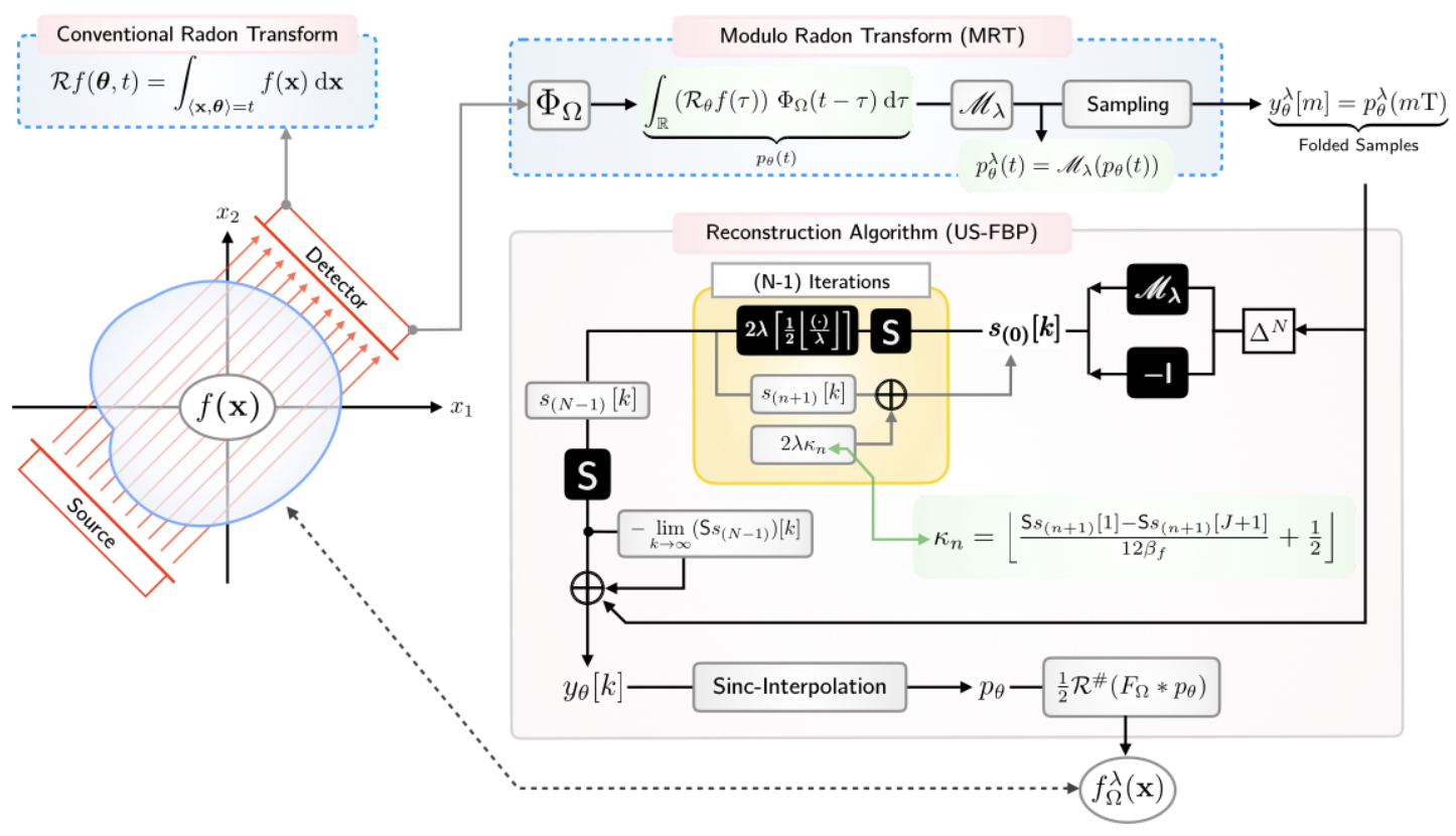
The US-CT is a single-shot HDR CT, based on modulo sampling.
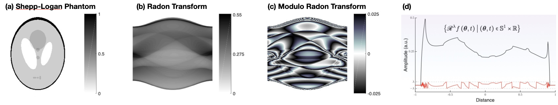
At the core of this approach stands the modulo Radon transform (MRT), arising from the hardware implementation of the system, where instead of recording the Radon projections, the modulo of Radon projections are computed and sampled.
The forward model of the US-CT can be written as,
Despite the non-linearity the many-to-one mapping due to the modulo operator, the MRT can be injective, and identifiable from semidiscrete MRT samples. This motivates the derivation of recovery conditions and algorithm.
The Inverse Problem.
To reconstruct an image, the MRT samples need to be inverted.
The conditions and algorithms that can be used for sampling that allows reconstruction can be classified based on the domain of operation.
Spatial-Domain Inversion. For a semi-discrete MRT model, where the angles are available on the continuum, exact recovery from MRT samples can be guaranteed under the given conditions.
Unlimited sampling–filtered back projection
Any \(f \in L^{1}(\mathbb{R}^2)\cap\mathcal{B}_{\Omega}(\mathbb{R}^2)\) can be uniquely recovered from semidiscrete MRT samples if \(T < 1 / \Omega\) and the reconstruction filter \(F_{\Omega}\) is chosen to be the Ram–Lak filter with window \(W = \mathbf{1}_{[-1,1]}\).
The recovery is based on US-FBP [17], a variant of the US-ALG.
In the case when \(f\) is not bandlimited but belongs to the more general Sobolev spaces of fractional order \(\alpha > 0\), given by \(H^{\alpha} (\mathbb{R}^2) = \bigl\{ f \in L^2(\mathbb{R}^2) \bigm| \| f \|_{\alpha} < \infty \bigr\}\), the reconstruction error using the US-FBP can be upper bounded.
If only finitely many time samples and angles are available, the image can be approximated based on a sequential application of modulo unfolding and a discrete FBP reconstruction formula.
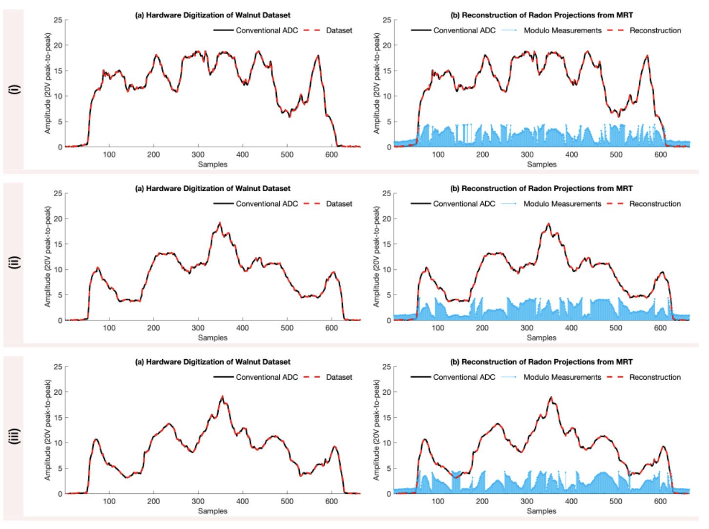
Hardware Experiment The proposed US-CT was experimentally tested using the M-ADC. In the experiment, and image from The Walnut Dataset was re-digitized using the M-ADC over \(20\) angles, and then algorithmically recovered.
The technique achieves a reconstruction error at the order of \(10^{-3}\), with dynamic range enhancement of \(AAAA\). The sampled waveforms and the reconstruction from modulo samples for a fixed angle are presented below.
Fourier-Domain Inversion
Implementing spatial-domain inversion poses several challenges for real-time applications.
These include the numerical instability when inverting higher differences, the high oversampling factor, and the need for prior knowledge of \(\lambda\).
A Fourier-domain approach offers advantages by harnessing a wide range of tomographic recovery techniques to address these issues. Yet, working with non-linearities is particularly difficult in the transform domain.
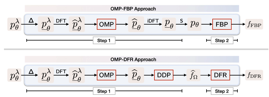
OMP-DFR
The first algorithm, OMP-DFR (Orthogonal Matching Pursuit - Direct Fourier Reconstruction), is a mixture of
a Fourier domain and spatial domain reconstruction approaches:
#. Reconstruction of the Fourier Radon samples based on a Fourier-domain separation principle (see US-FP) and a sparsity property. This is done using the OMP algorithm.
#. Reconstruction of the target function using filtered back projection formula.
The reconstruction in first part can be guaranteed, while the error due to the FBP can be bounded.