

Next: Performance on Novel Data
Up: Forward Models for Non-Convex
Previous: Training the Forward Model
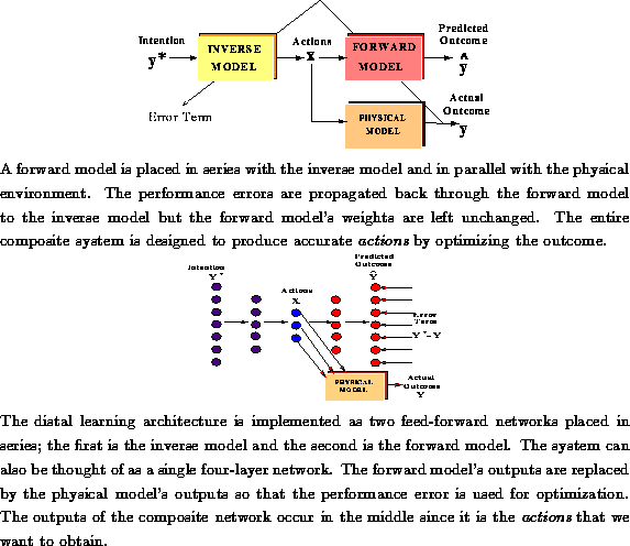
Once the forward model was trained we placed it in series with the
inverse model to form a composite learning system of the type
shown in Figure  . Again, the inverse model was
implemented as a two-layer feed-forward network with 61 input units,
20 logistic hidden units and 2 output units.
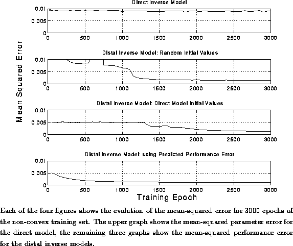
The composite model can also be thought of as a single four-layer
feed-forward network, see Figure
  . First the intention
waveform
  was given to the input units of the inverse
model. The activations were fed forward, through the inverse model, to
the forward model.
The activations passed completely through the four layers of the
network until values were obtained for the output of the forward model.
We then recursively computed the deltas for each of the 4 layers and
adjusted the weights of the inverse model, leaving the forward model
unchanged since it had already converged to a satisfactory solution.\

Figure: Connectionist Implementation of Composite Learning Scheme
Figure: Composite Learning Scheme
There are three approaches to training the inverse model using a
forward model: training from random initial conditions, training from
the direct inverse model's final condition and training with the
predicted performance error of Equation  .\
.\
Training from random initial conditions is standard practice for many
applications of connectionist networks. The strength of the connections are
initialized to small (  ) uniformly distributed
values with zero mean. As the network converges to a globally
satisfactory solution, the weights get larger, representing a progressively
higher-order fit to the training data. Initializing the network with small
weights ensures that the model does not over-fit the data.\
If we initialize the distal inverse model with the weights obtained from the
direct inverse model the task of the composite learning system is
made somewhat easier and we observe faster convergence than for random
initial conditions. This technique works because the direct
inverse model is good for convex regions of the solution space; if the
inverse modeling problem has relatively small non-convex regions the
difference between the direct inverse model and distal inverse model
will be small.\
We used the performance error for optimization during learning
with these models, see Equation  , which is different
than the predicted performance error of Equation
  .
.
However, we also obtained good results with faster convergence by using
the predicted performance error; the
difference was that the predicted performance error used the forward
model's outputs as an error measure so there was no need to present
the action parameters to the physical model.
An inverse model trained in this way is biased by
the inaccuracies of the forward model, thus we
switched to performance error optimization for the last few epochs of
training. This technique is only effective if the forward model has
converged to a good approximation of the physical model. We
initialized the inverse model with the direct inverse model's final
values. See Table  for a summary of the various
error functions and training sets that were used for the above models.\

Table: Training Sets and Error Terms for the Various Models
Figures  ,
,  and
and  show the results of training the inverse model
using the three forward-modeling strategies outlined above, as well as the
results for the direct inverse modeling technique.\

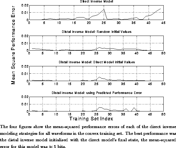
Figure: Convergence of the Inverse Models: Non-Convex Data

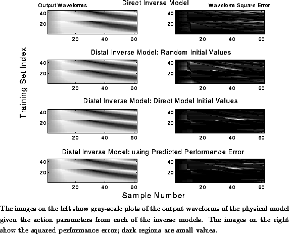
Figure: Mean Performance of the Inverse Models: Non-Convex Data

Figure: Performance Outcomes of the Inverse Models: Non-Convex Data
We can see from Figure  that the fastest
convergence was given by the the third of the non-direct techniques,
which used the predicted performance error for most of the training
epochs. After
3000 trials the three distal-inverse models had converged to a
solution that met the error criterion, the direct inverse model had
not.\
The mean-squared performance errors for the entire training set of the
two-string violin model are shown in Figure  .
The performance errors, shown in Figure
  , are
concentrated in smaller regions for the three distal-inverse models
than for the direct inverse model. The inverse model with the best overall
performance was the distal inverse model trained from the direct
inverse model's final values. The mean-squared performance
error for this model was
  which gives an accuracy
of bits. This is
significantly better performance than for the direct inverse model
and is well within the required criterion of 6 bits of error.\


Next: Performance on Novel Data
Up: Forward Models for Non-Convex
Previous: Training the Forward Model
Michael Casey
Mon Mar 4 18:10:46 EST 1996
 . Again, the inverse model was
implemented as a two-layer feed-forward network with 61 input units,
20 logistic hidden units and 2 output units.
The composite model can also be thought of as a single four-layer
feed-forward network, see Figure
  . First the intention
waveform