 .
.
Solution regions and learnability are well-studied characteristics
in the machine learning community; see for example,
[, , ]. A solution set X is said to
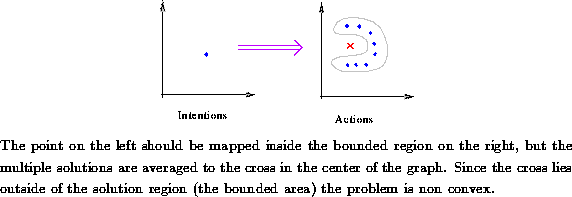
be convex if and only if there exist three co-linear points p,q,r
such that, if ![]() and
and ![]() , then
, then ![]() ; otherwise the region is
non-convex. See Figure
; otherwise the region is
non-convex. See Figure  .
.

Figure: Non-Convexity of One-to-Many Mappings
As an illustration of modeling a convex solution space we implemented an inverse model to learn to map a sound waveform, generated by a physical model of a single violin string, to the physical stop position on the string. This mapping was unique, and therefore convex, since for every sampled waveform that was produced using the physical model, there was only one stop-parameter value.\
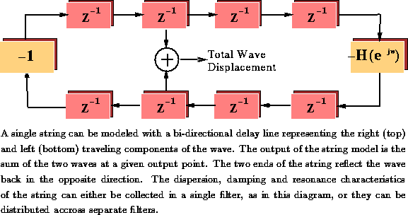
The violin string model was implemented using a discrete version of the
wave equation efficiently computed using digital waveguides and
linear time-invariant filters for damping, dispersion and resonance
characteristics: [, ], see
Figure  . The parameterization of the violin model
is given in Table
  .
.

Figure: Digital Waveguide Model of a String

Table: String Model Parameters
The first experiment required only the D string of the violin.
The length of the violin from the nut to the bridge was 0.32 m
and the model was calibrated so that the pitch class A4 was at
440.000 Hz, thus the open D string had a fundamental frequency of
![]() Hz. The speed of wave propagation in the string was
determined by
Hz. The speed of wave propagation in the string was
determined by ![]() where K
was the string tension and
where K
was the string tension and ![]() was the linear mass density of the
string; for the D string the wave propagation speed was 187.9456 m/s.\
was the linear mass density of the
string; for the D string the wave propagation speed was 187.9456 m/s.\
The training set for the direct inverse model comprised a set of time-domain
waveforms generated by the violin model, ![]() , and a set of
target parameters that produced the waveforms,
, and a set of
target parameters that produced the waveforms, ![]() . The
original waveforms were represented at 16-bit resolution with floating-point
values in the range 0-1. We used the first 61 samples generated by the
physical model as the representative set for each of the waveforms;
this allowed frequencies as low as 293.665 Hz (D4) to be uniquely
represented. The waveforms were generated at frequencies spaced a
half-step apart along the D string, spanning two octaves starting in
open position (0.32 m). The stop position for each
of the waveforms was expressed as distance along the string.\
. The
original waveforms were represented at 16-bit resolution with floating-point
values in the range 0-1. We used the first 61 samples generated by the
physical model as the representative set for each of the waveforms;
this allowed frequencies as low as 293.665 Hz (D4) to be uniquely
represented. The waveforms were generated at frequencies spaced a
half-step apart along the D string, spanning two octaves starting in
open position (0.32 m). The stop position for each
of the waveforms was expressed as distance along the string.\
The direct inverse model was implemented as a two-layer feed-forward network
with biases, utilizing the generalized delta-rule as a learning algorithm,
[]. There were 61 linear input units, one for each sample of the
sound intention ![]() , 20 logistic hidden units and a single
linear output unit for the stop position. The training pairs were
presented in random order with the entire set of data being presented
in each epoch. We used an adaptive learning-rate strategy and included
a momentum term for faster convergence.
, 20 logistic hidden units and a single
linear output unit for the stop position. The training pairs were
presented in random order with the entire set of data being presented
in each epoch. We used an adaptive learning-rate strategy and included
a momentum term for faster convergence.

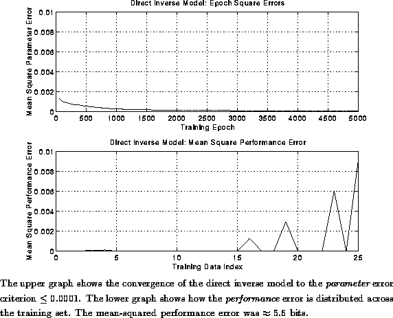
Figure: Convergence and Mean Errors of Direct Inverse Model: Convex Data
Figure  shows the convergence of the parameter
errors in the inverse model for 5000 epochs of the training data, and
the mean-squared performance error for each of the training patterns after the
inverse model reached criterion. The parameter error is the
difference between the target actions
 ![]() and the
output of the inverse model
and the
output of the inverse model ![]() :
:
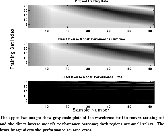
The performance waveforms and the squared performance errors are shown in
Figure  . The performance outcome was computed by
applying the outputs of the inverse model
 ![]() to the inputs
of the physical model. The performance error compares the
the input waveform
to the inputs
of the physical model. The performance error compares the
the input waveform ![]() to the outcome waveform
to the outcome waveform ![]() :
:
The mean-squared performance errors are given by:
where N is the number of training patterns, M is the number of samples in the waveform.

Figure: Performance Outcome of Direct Inverse Model: Convex Data
The original waveforms had 16 bits of resolution; the mean-squared
performance error of the direct inverse model after convergence to
criterion was ![]() . The accuracy of the performance was given
by bits. This was the
performance accuracy of the inverse model when trained to a mean
square parameter accuracy of
. The accuracy of the performance was given
by bits. This was the
performance accuracy of the inverse model when trained to a mean
square parameter accuracy of ![]() . The accuracy
of the direct inverse model of the convex data set was acceptable for
our purposes. (The typical noise margin for digital recording
. The accuracy
of the direct inverse model of the convex data set was acceptable for
our purposes. (The typical noise margin for digital recording ![]() bits).\
bits).\
The evaluation of the model in this manner was purely a matter of convenience for illustration purposes. If we were interested in developing a perceptual representation of auditory information we would not use the error critereon cited above, which reflects the ability of the system to reconstruct the original data. For more sophisticated applications of inverse modeling for audio data, we would need to develop perceptual error measures, ensuring that the machine makes judgements that are perceptually valid in human terms; see, for example, [, ]. \