By adding another degree of freedom to the violin string model we made
the task of
learning the inverse model a much harder problem. In the next
experiment we added a second string; the
learning task was to map a set of waveforms to
parameters representing the string stop positions (as in the
previous experiment) as well as a unit representing string selection, in this
case the D string ( ![]() Hz) and the A string (
Hz) and the A string ( ![]() Hz). In the physical-model implementation, the fundamental
pitch
Hz). In the physical-model implementation, the fundamental
pitch ![]() of each string
in open position was determined by the speed of propagation of the wave
through the string,
of each string
in open position was determined by the speed of propagation of the wave
through the string, ![]() . For the D
string the speed of propagation was 187.9456 m/s and for the A
string it was 281.6000 m/s.\
. For the D
string the speed of propagation was 187.9456 m/s and for the A
string it was 281.6000 m/s.\
The set of stop positions spanned two octaves for the D string
(D3-D5) and an augmented eleventh for the A string ( ![]() )
spaced at half-step intervals.
The pitch ranges were determined by the resolution of the
physical model since it was implemented as a digital waveguide with
unit delays. The highest frequency for half-step resolution,
without adding fractional delays to the
model, is given by
)
spaced at half-step intervals.
The pitch ranges were determined by the resolution of the
physical model since it was implemented as a digital waveguide with
unit delays. The highest frequency for half-step resolution,
without adding fractional delays to the
model, is given by ![]() , where SR is
the sampling rate of the physical model and n is
the number of delays used to model the string. The minimum number of
delays required for a half-step resolution has to satisfy the
inequality:
, where SR is
the sampling rate of the physical model and n is
the number of delays used to model the string. The minimum number of
delays required for a half-step resolution has to satisfy the
inequality:
This gave ![]() for the required half-step interval resolution.
The sample rate was 44100 Hz, thus the highest frequency was 1297.1
Hz, approximately
for the required half-step interval resolution.
The sample rate was 44100 Hz, thus the highest frequency was 1297.1
Hz, approximately ![]() .\
.\
There was considerable overlap in the training data because the waveforms from the string model for pitch classes A4-D5 on both strings were exactly equivalent. With this overlap the solution space was non-convex; thus solutions that averaged the multiple parameter sets for each duplicated waveform were not valid.\
To show how this applies to the problem of inverse modeling we used
the direct inverse modeling strategy of Section  on
the the non-convex training data.
Figures
  and
and  show the results obtained using the two-layer feedforward network
described above, with an extra output unit representing the choice of string.
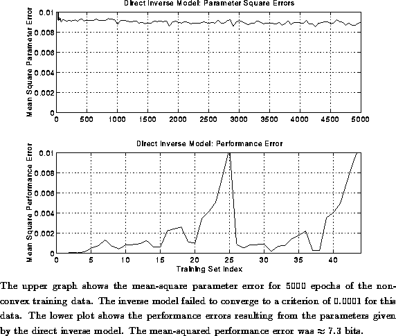
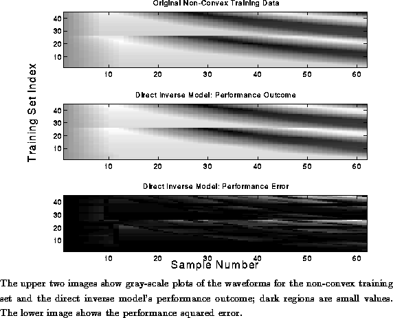
The model failed to converge to criterion over 5000 epochs, so the
performance error was significant in some regions of the solution space.
The mean-squared performance error was 0.0024; using the same calculation for
the accuracy as for the convex data set we got bits of error, which was significantly worse performance
than for the convex data set.\

Figure: Convergence and Mean Errors of Direct Inverse Model: Non-Convex Data

Figure: Performance Outcome of Direct Inverse Model: Non-Convex Data
These results show that direct inverse modeling using a two-layer feed-forward network gave unsatisfactory results for non-convex training data. We improved on the accuracy of the inverse model by implementing a learning technique that was better suited to non-convex data set.\