Day 37 - Multivariate clustering
Last time we saw that PCA was effective in revealing the major subgroups of
a multivariate dataset. However, it is limited by what can be seen in a
two-dimensional projection. Sometimes the group structure is more complex
than that. A more general way to break a dataset into subgroups is to use
clustering. Geometrically, clustering tries to find compact and
well-separated point clouds within the overall cloud. The methods for
multivariate clustering are similar to those discussed on day9, but with some new twists.
Ward's method
Previously we used a sum of squares criterion for clustering, with the
option to get a hierarchy (Ward's method) or a partitioning (k-means). How
do we assess the quality of a multivariate clustering? Using the
definition of distance from day35, we can construct
a generalized sum of squares criterion: SS = sum_{clusters j}
sum_{points i in j} ||x_i - m_j||^2 Ward's method works by making
each point a cluster, then merging clusters in order to minimize the sum of
squares. The merging cost that results from the sum of squares criterion
is na*nb/(na+nb)*||a - b||^2, a simple generalization of the
merging cost in the one-dimensional case. Iterative reassignment is also
possible using this sum of squares criterion, giving a multivariate k-means
algorithm. The commands to use in R are hclust and
kmeans.
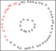
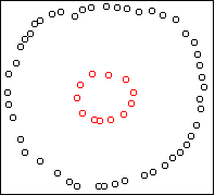
Here is an example two-dimensional dataset:
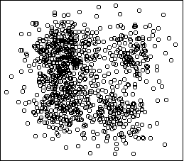
hc <- hclust(dist(x)^2,method="ward")
plot.hclust.trace(hc)
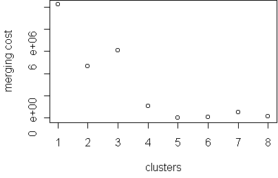
The merging trace shows that 4 is an interesting number.
Given the desired number of clusters, the function cutree
will cut the tree and return a vector telling you which cluster each case
falls into. We will save this in the data frame as an additional variable,
allowing us to make a cplot:
x$cluster <- factor(cutree(hc,k=4))
cplot(x)
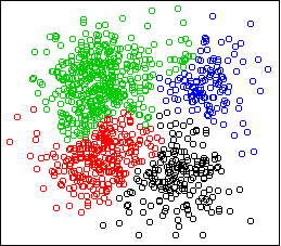
The sum of squares criterion desires separation
and balance. The merging cost prefers to merge small clusters
rather than large clusters, given the same amount of separation. In the
multivariate case, sum of squares also wants the clusters to be spherical;
it does not want highly elongated clusters. This is because distance is
measured equally in all directions. Counterintuitive
clusterings can result from this property.
Consider this two-dimensional dataset:
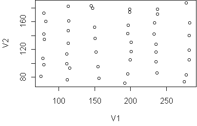
The data falls into six vertical strips.
This can easily happen when the clusters are compact in one
dimension (horizontal) and highly variable in another (vertical).
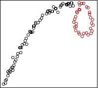
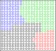
Here is the result of Ward's method, 6 clusters:
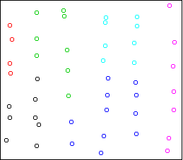
The clusters are chosen to be small and round, in violation of the
structure of the data.
Single-link clustering
This property of the sum of squares criterion has caused people to search
for alternatives. An extreme alternative is known as single-link
(or nearest-neighbor) clustering. It is a merging algorithm: you
start with all points in separate clusters, and repeatedly merge the two
closest clusters. The difference is in how the distance between clusters
is measured. Instead of using the distance between means, as Ward's method
does, it uses the distance between the two closest points from each
cluster, i.e. the size of the gap between the clusters. This algorithm has
no preference for spherical clusters or any other shape. It does not scale
the distance by cluster size, so it doesn't prefer balance either.
It is extreme among clustering algorithms in that it only desires separation.
You can switch to single-link clustering by telling
hclust to use method="single".
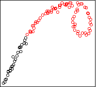
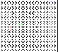
Here is the result on the strips data:
hc <- hclust(dist(x)^2,method="single")
x$cluster <- factor(cutree(hc,k=6))
cplot(x)
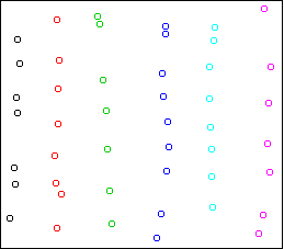
It divides the data into the six strips.
However, the blind pursuit of separation can also lead to counterintuitive
clusterings.
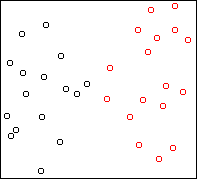
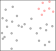
Here is the result on the first example above, showing the
k=5 solution:
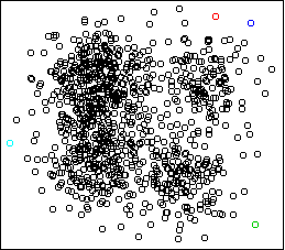
Four outlying data-points have been assigned their own cluster, and the
rest of the data in the middle, which is very dense, has been lumped into
the remaining cluster. Single-link can do this because it doesn't care
about balance.
Here are some more examples:
Cars
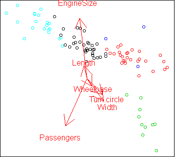
Let's compare clustering to PCA on the car dataset.
Here is the PCA projection, with points colored by cluster:
sx <- scale(x)
w <- pca(sx,2)
hc <- hclust(dist(sx)^2,method="ward")
sx$cluster <- factor(cutree(hc,k=5))
cplot(project(sx,w))
plot.axes(w)
The clusters follow the PCA projection pretty closely, even though the
clusters were computed in the full 10-dimensional space, not the
2-dimensional projection. The only difference from our analysis on day36 is that the cars with high MPG have been divided
into two groups, corresponding to compact and midsize cars.
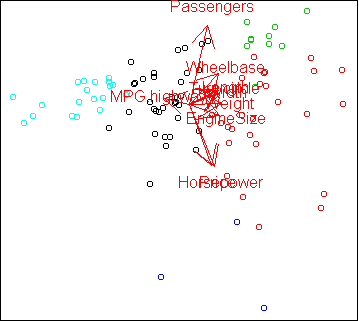
Another way to view the result of clustering is to treat the clusters
as classes and make a discriminative projection:
x$cluster <- factor(cutree(hc,k=5))
w2 <- projection(x,2)
cplot(project(x,w2))
plot.axes(w2)
The projection is a little odd in that the seemingly most important
variables like Horsepower and MPG are not used.
projection found a different set of variables which can also
separate the clusters.
States
Here is the PCA projection of the states data, colored by cluster:
sx <- scale(x)
w <- pca(sx,2)
hc <- hclust(dist(sx)^2,method="ward")
sx$cluster <- factor(cutree(hc,k=4))
cplot(project(sx,w))
plot.axes(w)
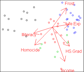
In this case, the clustering does not completely agree with PCA.
The green class is split up and one red point is far from its cluster.
Here is the discriminative projection:
x$cluster <- factor(cutree(hc,k=4))
w2 <- projection(x,2,type="m")
cplot(project(x,w2))
plot.axes(w2)
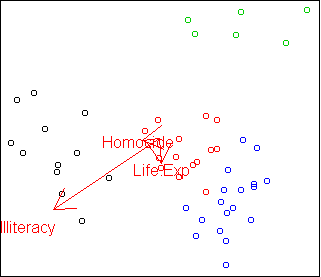
Only the three variables Life.Exp, Illiteracy, and
Homocide are needed to distinguish the clusters.
This projection shows that the green cluster is most unusual compared to
the other three.
We will examine this more closely in the next lecture.
Code
To use these functions, you need the latest version of
clus1.r
clus1.s
Functions introduced in this lecture:
- hclust
- plot.hclust.trace
- cutree
Tom Minka
Last modified: Mon Aug 22 16:41:25 GMT 2005