Day 9 - Numerical abstraction by clustering

So far we have covered two principles for abstraction: balance and density-preservation. Today we discussed in detail a third principle, which is to preserve distinctions within a dataset. The idea is to look for compact and separated subgroups in the data, a process which is called clustering.

After considering a few examples, it becomes clear that separation alone is not a sufficient criterion for clustering. Separation reveals itself as valleys in the histogram. If the dataset is uniformly distributed among its range, there are no valleys and thus no separation. But it wouldn't be right to put everything into one cluster, one abstraction bin, since that would not "preserve distinctions." The dataset could be composed of two very different subgroups, whose density along this variable happens to be uniform. In the uniform case, the natural binning is an equally spaced one. It preserves the distinction between distant points but not between nearby points. We can explain this as a desire for balance as well as separation. There are many choices for how to trade-off balance and separation. Today we discuss one way.

The choices we have when clustering can be broken down as follows:

Which clustering criterion to use
What type of output do we want
How do we optimize the criterion

The first choice is how do we want to trade-off balance and separation. The second choice is whether we want a single partition of the data in k bins or whether we want a hierarchy of nested partitions from which we choose later. The third choice is whether we use a merging algorithm, iterative reassignment, or something else.

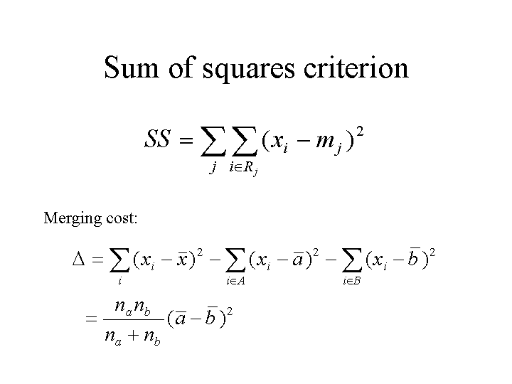
A criterion which achieves a nice trade-off of balance and separation is the sum-of-squares criterion. The evaluate a given clustering, we compute the mean of the data in each cluster, then add up the sum of squared differences between each point and its cluster mean. Note that this is just the variance of the cluster times the size of the cluster, summed over all clusters. We want to minimize the criterion, i.e. a large sum of squares is bad. This criterion clearly wants clusters to be compact. It also wants balance, because big clusters cost more than small ones with the same variance.

Ward's method

There are several ways to implement this criterion. One way is to start with each point in a cluster by itself (sum of squares = 0) and successively merge clusters in order to minimize the increase in the sum of squares. This is called "Ward's method" and is very similar to algorithm B for balancing. You just consider what happens to the sum of squares when two clusters are merged. This "merging cost" turns out to have a simple formula which is the difference between the cluster centers times the size of the clusters. The tradeoff between separation and balance is evident in this formula. For clusters which are the same distance away, it is better to merge the smaller ones. Consider the case where one cluster is just a single point. It wants to join not just the closest cluster but one with a small number of points already in it. Ward's method can give a hierarchy or a partition. If you want a partition, just stop when you reach k bins.

K-means

Another way to minimize the sum-of-squares is by iterative re-assignment. You guess an initial clustering and then repeatedly re-assign points between clusters. To re-assign a point, you compute how the sum of squares would change if you put this point in another cluster. If the sum of squares would go down, you make the re-assignment. The change in the sum of squares is the cost of merging the point with another cluster minus the cost of merging with the cluster it is already in (you are regaining that cost). This algorithm is very efficient. It is also incremental in that you can take in new data and dynamically adjust the clustering appropriately. With Ward's method, you would have to start from the bottom and make the tree all over again. Iterative re-assignment and its variations are collectively called "k-means" algorithms, since they work with a fixed set of k means that move around by changing cluster assignments. k-means always produces a sum of squares which is lower than Ward's method for the same number of bins, because it is not restricted to produce nested binnings. Ward's method tends to produce less balanced and more separated clusters.

A disadvantage of k-means algorithms is that the answers they give are not unique. While there may be only one clustering with minimum sum of squares, these algorithms will not necessarily find it every time. Iterative re-assignment is a local search algorithm: it makes small changes to the solution and sees if the objective got better. Local search is also called hill-climbing, by analogy to an impatient hiker who tries to find the highest peak by always walking uphill. This strategy can stop at local minima, where the criterion is not optimized but no improvement is possible by making small changes. Which local minimum you stop at depends on where you were when you started. Hence the k-means algorithms give different results depending on how they make their initial guess. A typical initial guess is to pick k data points at random to be the means.

Code

You need to download and source these files before you can use clustering commands in R or S.

clus1.r clus1.s
Class examples

Two routines are provided for getting a set of bin breaks according to one of the above schemes. The function break.hclust(x,n) uses Ward's method to divide the range of x into n bins. It plots the breaks and returns a break vector, just like bhist.merge. It also gives a trace of the cost of each merge. This allows you to choose the number of clusters. An interesting number of clusters is one which directly precedes a sudden jump in merging cost.

The function break.kmeans(x,n) does the same thing but with k-means. Note that break.kmeans does not always give the same answer every time you run it.

If you want a full hierarchy, you can use the built-in function hclust. It returns a hierarchy object that you can view as a tree using plot in R or plclust in S. You can also view it as a nested set of bin breaks using plot.hclust.breaks. See the example code.

Optional reading

Clustan is a company which sells clustering software. Check out their interesting case study of k-means clustering for data mining, as well as their critique of k-means.

Tom Minka

Last modified: Mon Dec 17 14:28:52 EST 2001