Unlimited Sensing Framework
Reproducible Research: Code+Data+Hardware Link
\[ \require{amssymb ,mathrsfs} \require{mathrsfs} \def\Z{\in \mathbb{Z}} \def\R{\in \mathbb{R}} \def\iC{\in \mathbb{C}} \newcommand{\PW}[1]{\mathsf{PW}_{#1}} \def\T{\mathrm{T}} \def\B{\beta_g} \def\DR{\mathsf{DR}} \def\kn{\kappa_{\l \ell \r}} \def\S{\mathsf{S}} \def\bo{b_0} \newcommand{\rob}[1]{\left( #1 \right)} \def\dtft{\hat{\mathrm{C}}\rob{\w}} \def\dtftm{\hat{\mathrm{C}}_m\rob{\w}} \newcommand{\cmi}[1]{\hat{\mathrm{C}}_{m_{#1}}\rob{\w}} \newcommand{\cmc}[1]{\hat{\mathrm{C}}^*_{m_{#1}}\rob{\w}} \newcommand{\gram}[1]{\mathsf{G}^{\rob{#1}}_{m_1,m_2}\rob{\w}} \newcommand{\todo}[1]{\hl{\sf\small{#1}}} \newcommand{\bs}[1]{\boldsymbol{#1}} \newcommand{\ft}[1]{\left[\kern-0.15em\left[#1\right]\kern-0.15em\right]} \newcommand{\fe}[1]{\left[\kern-0.30em\left[#1\right]\kern-0.30em\right]} \newcommand{\flr}[1]{\left\lfloor #1 \right\rfloor} \newcommand{\MO}[1]{\mathscr{M}_\lambda\l #1 \r} \newcommand{\VO}[1]{\varepsilon_{#1}} \newcommand{\ab}[1]{{\color{red} #1}} \newcommand{\sqb}[1]{\left[ #1 \right]} \def\l{\left(} \def\r{\right)} \newcommand{\todo}[1]{\hl{\sf\small{#1}}} \newcommand{\bs}[1]{\boldsymbol{#1}} \newcommand{\ft}[1]{\left[\kern-0.15em\left[#1\right]\kern-0.15em\right]} \newcommand{\fe}[1]{\left[\kern-0.30em\left[#1\right]\kern-0.30em\right]} \newcommand{\flr}[1]{\left\lfloor #1 \right\rfloor} \newcommand{\MO}[1]{\mathscr{M}_\lambda\l #1 \r} \newcommand{\VO}[1]{\varepsilon_{#1}} \newcommand{\ab}[1]{{\color{red} #1}} \newcommand{\sqb}[1]{\left[ #1 \right]} \newcommand{\rob}[1]{\left( #1 \right)} \def\l{\left(} \def\r{\right)} \newcommand{\conv}{\mathop{\scalebox{1}{\raisebox{0ex}{\(\circledast\)}}}}% \def\sdh{\circledast_h} \def\sdH{\circledast_{\mat{H}}} \def\sd{\circledast} \newcommand{\mat}[1]{\mathbf{#1}} \def\Hi{\mathbf{H}^{-1}} \newcommand{\EQc}[1]{\stackrel{(\ref{#1})}{=}} \def\YN{{\color{black}y _{\eta}}} \def\DO{N} \def\Do{n} \newcommand{\lp}[1]{{\ell}_{#1}} \newcommand{\Lp}[1]{\mathbf{L}_{#1}} \newcommand{\normt}[3]{ {\| {#1} \|}_{ {\mathbf{L}_{#2}} \left( #3\right)}} \newcommand{\normT}[3]{ {\| {#1} \|}_{ {\boldsymbol{\ell}_{#2}} \left( #3\right)}} \newcommand{\fk}[1]{{\mathsf{F}}_{#1}} \def\e{\mathrm{e}} \]
Imagine capturing signals clearly and precisely—no matter how faint or powerful they are. Conventional digital systems often struggle, losing details when signals become too strong or too subtle. The Unlimited Sensing Framework (USF) provides an original, better approach.
USF (US10651865B2) introduces a revolutionary paradigm in digital sensing and signal processing by intentionally leveraging quantization noise, traditionally viewed as unwanted error, to effectively capture signals with exceptional dynamic range and digital resolution.

Consider the analogy of wrapping a long strand of spaghetti around a fork. Similarly, USF employs innovative hardware to fold high dynamic range (HDR) signals within the analog domain, preventing saturation and preserving critical signal features without sacrificing digital resolution.
At the core of USF lies an original mathematical insight: for smooth signals, the fractional part (quantization noise) encodes the integer part (the quantized signal).
In crux, USF enables signal recovery from quantization noise (modulo samples) at constant-factor Nyquist-rate. After digital acquisition, specialized mathematical algorithms decode these folded signals, reconstructing them with HDR and digital precision.
For a fix bit-budget, the USF simultaneously offers HDR signal recovery with high digital resolution which is not possible with conventional ADCs. This novel approach transforms what was once considered noise into valuable data, enabling a new sensing technology.
Sensing Model
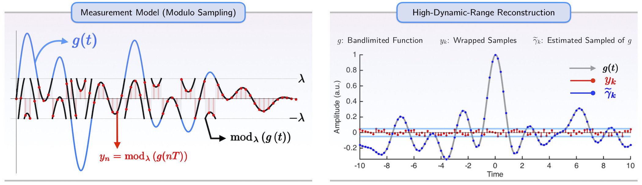
The key novelty of our approach is that instead of (potentially clipped) pointwise samples of the bandlimited function, we work with folded amplitudes with values in the range \(\left[ { - \lambda ,\lambda } \right]\). Mathematically, this folding corresponds to injecting a non-linearity in the sensing process. This amounts to,
\[ \begin{equation} \mathscr{M}_{\lambda}:f \mapsto 2\lambda \left( {\fe{ {\frac{f}{{2\lambda }} + \frac{1}{2} } } - \frac{1}{2} } \right), \label{map} \end{equation} \]
where \(\ft{f} = f - \flr{f} \) defines the fractional part of \(f\) and \(\lambda>0\) is the ADC threshold. Note that \(\eqref{map}\) is equivalent to a centered modulo operation. By implementing the mapping \(\eqref{map}\), it is clear that out-of-range amplitudes are folded back into the dynamic range \(\left[ { - \lambda ,\lambda } \right]\). This is shown in Fig:1.
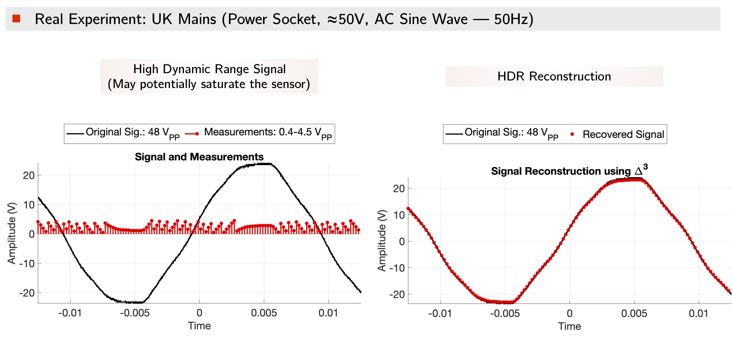
Example of Real Experiment
To appreciate the practical utility of the Unlimited Sampling strategy, here we show an experiment based on our prototype hardware. We show that voltages from the UK Mains (power socket, 50V) can be stored and reconstructed on a digital device such as a µ-controller or a MacBook. This cannot be possible using any existing, digitizing technology which will either saturate or crash.
Recovery — A First Result: The Unlimited Sampling Theorem
Recovery Conditions
In analogy to Shannon’s sampling theorem, our first result [1], the Unlimited Sampling Theorem proves that a bandlimited signal can be recovered from modulo samples provided that a certain sampling density criterion, that is independent of the ADC threshold, is satisfied. In this way, our result allows for perfect recovery of a bandlimited function whose amplitude exceeds the ADC threshold by orders of magnitude.
Theorem (BKR, 2017 [1]) Let \(f(t)\) be a function with no frequencies higher than \(\Omega\) (rad/s), then a sufficient condition for recovery of \(f(t)\) from its modulo samples \(y_k = \MO{f(t)}, t = kT\), \(k\in\mathbb{Z}\) is,
\[ \begin{equation} T \leq \frac{1}{2\Omega e}. \label{TUS} \end{equation} \]
Uniqueness Conditions
In fact, there is a one-to-one mapping between a bandlimited function and its modulo samples provides that the sampling rate is higher than the critical rate of the Nyquist rate, \(T<\pi/\Omega\). The Injectivity Conditions are proved in [2].
Theorem (BK, 2019 [2]) Let \(f(t)\) be a finite-energy function with no frequencies higher than \(\Omega\) (rad/s). Then the function \(f(t)\) is uniquely determined by its modulo samples \(y_k = \MO{f(t_k)}\) taken on grid \(t = kT_\epsilon\), \(k\in\mathbb{Z}\) where
\[ 0<T_\epsilon< \frac{\pi}{\Omega+\epsilon}, \quad \epsilon>0. \]
Bounded Noise and Quantization
When working with bounded noise, we assume that the modulo samples \(y[k]\) are affected by noise \(\eta\) of amplitude bounded by a constant \( \bo > 0\). That is,
\[ \begin{equation} \forall k \Z, \quad \YN\left[ k \right] = y[k] + \eta\left[ k \right], \quad \left| {\eta \left[ k \right]} \right| \leqslant {\bo}. \end{equation} \]
Note that due the presence of noise, it may happen that \(\YN [k] \not\in [-\lambda,\lambda]\). Nonetheless, for \(\bo\) below some fixed threshold, our recovery method provably recovers noisy bandlimited samples \(\gamma[k]\) from the associated noisy modulo samples \(\YN[k]\) up to an unknown additive constant, where the noise appearing in the recovered samples is in entry-wise agreement with the one affecting the modulo samples. That is, \(\widetilde \gamma \left[ k \right] = \gamma \left[ k \right] + \eta \left[ k \right] + 2m\lambda, m\in \mathbb{Z}\).
Theorem (BKR, 2020 [3]) Let \(g\l t\r\) be an \(\Omega\)-bandlimited and finite-energy signal. Assume that \(\B\in 2\lambda \mathbb{Z}\) is known with \(\|g\|_\infty\leqslant \B\). For the dynamic range we work with the normalization \(\DR = {\B}/{\lambda}\). Let the noisy modulo samples with a noise bound given in terms of the dynamic range as,
\[ \begin{equation} \label{eq:mns} \left\| \eta \right\|_\infty \leqslant \tfrac{\lambda }{4}{\left( {{{2\cdot\DR}}} \right)^{ - \frac{1}{\alpha}}}, \qquad \alpha \in \mathbb{N}. \end{equation} \]
Then a sufficient condition for approximate recovery of the bandlimited samples \(\gamma[k]\) is that,
\[ \begin{equation} \label{MSBN} T \leqslant \frac{1}{2^\alpha \Omega e}. \end{equation} \]
The recovery is approximate in the sense that, \(\widetilde \gamma \left[ k \right] = \gamma \left[ k \right] + \eta \left[ k \right] + 2m\lambda, m\in \mathbb{Z}\).
Wider Classes of Inverse Problems and Function Spaces
Physical models arising in sciences and engineering are typically modeled as a linear system of equations, namely, \(\mat{y} = \mat{Ax}\). In the context of our work, the modulo non-linearity results in a wider class of inverse problems,
\[ y\rob{t} = \MO{\mathcal{A} x\rob{t}} \]
where \(\mathcal{A}\) is a continuous operator (e.g. low-pass filter or Radon transform) and the goal is to recovery \(x\) from sampled measurements \(y\).
Example 1: High Dynamic Range Imaging
To facilitate imaging beyond the conventional dynamic range, often referred to as high-dynamic-range (HDR) imaging, several algorithmic and hardware solutions have been proposed in the literature. These approaches rely on oversampling. The most common algorithmic solution is to fuse multiple images at different exposures
(Debevec (1997)). Hardware-only solutions use multiple ADCs and are exorbitantly priced. For instance, state-of-the-art ALEV III CMOS sensor designed by ARRI (for cinematography) uses Dual Gain Architecture. As the name suggests, each pixel simultaneously reads information with high and low amplification factors corresponding to clipped and non-clipped values, respectively. Both read-outs are fed to a \(14\)-bit ADC and combined into a single \(16\)-bit HDR image.
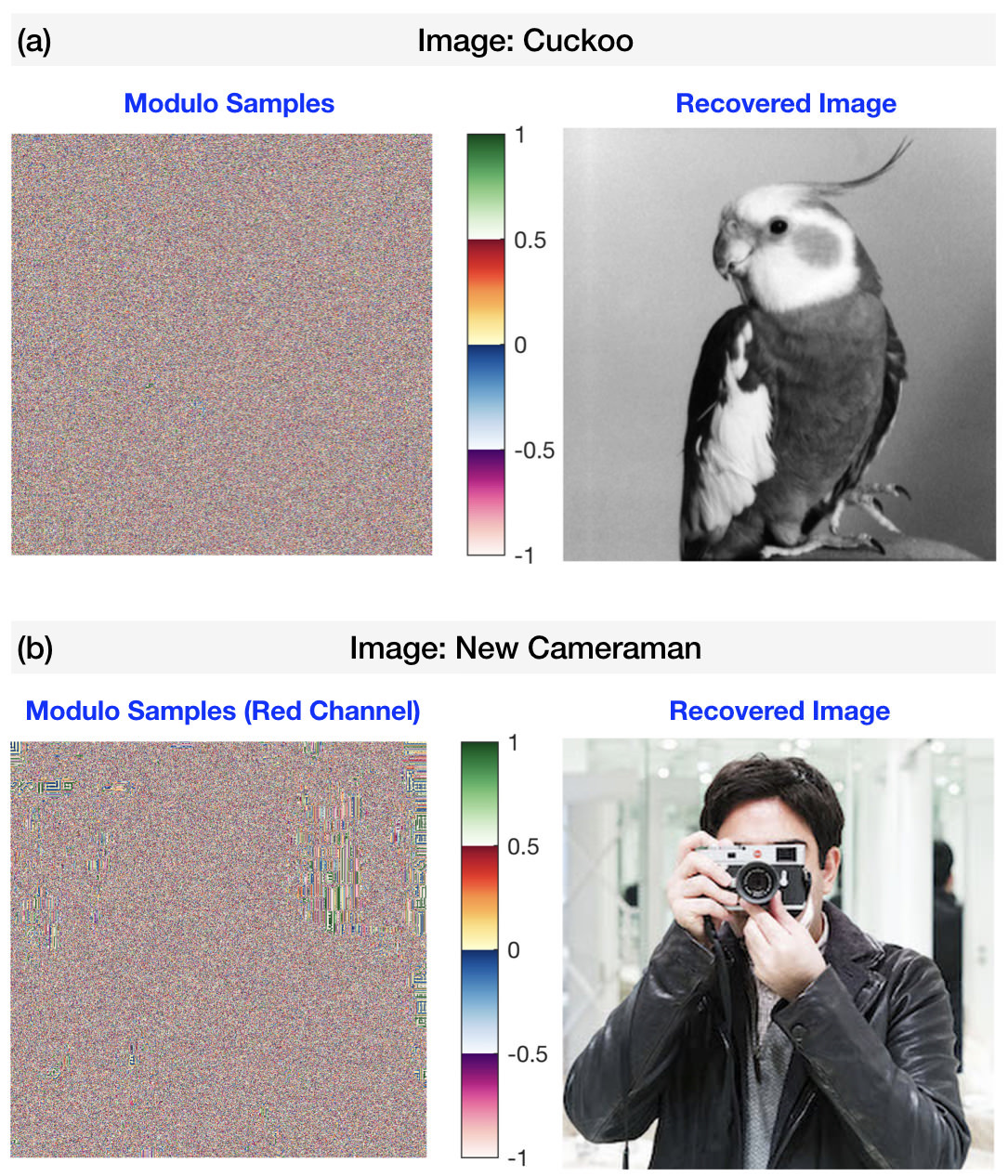
As we have pointed out earlier, HDR sensing is an in-built feature of the Unlimited Sensing architecture. However, images are non-bandlimited functions and hence the existing results do no apply. To overcome this bottleneck, we model images as objects in the shift-invariant space spanned by B-splines. Our main result is as follows. For any image \(g\l x \r \in {\sf{V}}_h^\DO \cap \Lp{\infty}\l \mathbb{R} \r \) where \({\sf{V}}_h^\DO\) is the space generated by shifts of B-splines of order \(\DO\) and refinement \(h\), it one has that,
\[ \begin{equation*} \label{MR} \normT{\Delta^\Do \gamma}{\infty}{\mathbb{R}} \leqslant \l\frac{T\pi \e}{h}\r^\Do \l \frac{\fk{\DO-\Do}}{\fk{\DO}} \r \normt{g}{\infty}{\mathbb{R}} , \quad \Do = 0,\ldots,\DO, \mbox{ where } \forall \ \DO \geq 0, \ \ {\mathsf{F}_N = \frac{4}{\pi } {\sum\limits_{k \geq0} \rob{\frac{\rob{-1}^k}{2k+1}}^{N + 1}}} \in \sqb{1,\frac{\pi}{2}}. \end{equation*} \]
The implication is that as shown in [4], the sampling rate,
\[ T < \frac{h}{{\pi e}}{\left( {\frac{\lambda }{{{{\left\| g \right\|}_\infty }\mathsf{C}_{\Do,\DO}}}} \right)^{\frac{1}{\Do}}}, \qquad \mathsf{C}_{\Do,\DO} = \frac{\fk{\DO-\Do}}{\fk{\DO}} \]
guarantees recovery of images modeled by splines. Examples of HDR imaging are shown below.
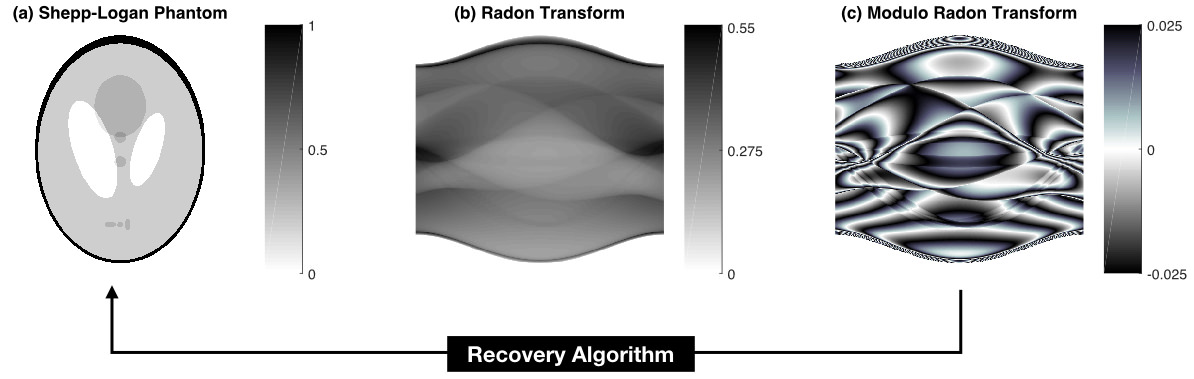
Example 2: Modulo Tomography
Recent advances in hardware have led to high dynamic range solutions for computed tomography. However, much in the same way as conventional imaging, HDR tomography requires fusion of multiple, calibrated Radon Transform projections. The inherent HDR feature of the modulo non-linearity can be leveraged in this context. To this end, we recently introduced the *Modulo Radon Transform in [6] and practical algorithm for HDR tomography was proposed in [7]. An example of the new approach is shown below.
References
Journals
Fourier-Domain Inversion for the Modulo Radon Transform
M. Beckmann, A. Bhandari and M. Iske
IEEE Transactions on Computational Imaging, (Apr. 2024).\(\lambda\)-MIMO: Massive MIMO via Modulo Sampling
Z. Liu, A. Bhandari and B. Clerckx
IEEE Transactions on Communications, (Aug. 2023).Unlimited Sampling of Bandpass Signals: Computational Demodulation via Undersampling
G. Shtendel, D. Florescu and A. Bhandari
IEEE Transactions on Signal Processing, (Sep. 2023).The Modulo Radon Transform: Theory, Algorithms, and Applications
M. Beckmann, A. Bhandari and F. Krahmer
SIAM Journal on Imaging Sciences, (Apr. 2022).Back in the US-SR: Unlimited Sampling and Sparse Super-Resolution With Its Hardware Validation
A. Bhandari
IEEE Signal Processing Letters, (Mar. 2022).Computational Array Signal Processing via Modulo Non-Linearities
S. Fernandez-Menduina, F. Krahmer, G. Leus and A. Bhandari
IEEE Transactions on Signal Processing, (Jul. 2022).Time Encoding via Unlimited Sampling: Theory, Algorithms and Hardware Validation
D. Florescu and A. Bhandari
IEEE Transactions on Signal Processing, (Sep. 2022).The Surprising Benefits of Hysteresis in Unlimited Sampling: Theory, Algorithms and Experiments
D. Florescu, F. Krahmer and A. Bhandari
IEEE Transactions on Signal Processing, (Jan. 2022).Unlimited Sampling from Theory to Practice: Fourier-Prony Recovery and Prototype ADC
A. Bhandari, F. Krahmer and T. Poskitt
IEEE Transactions on Signal Processing, (Sep. 2021).On Unlimited Sampling and Reconstruction
A. Bhandari, F. Krahmer and R. Raskar
IEEE Transactions on Signal Processing, (Dec. 2020).
Conferences
Dual-Channel Unlimited Sampling for Bandpass Signals
G. Shtendel and A. Bhandari
IEEE Intl. Conf. on Acoustics, Speech and Signal Processing (ICASSP), (Apr. 2024).Frequency Estimation via Sub-Nyquist Unlimited Sampling
Y. Zhu, R. Guo, P. Zhang and A. Bhandari
IEEE Intl. Conf. on Acoustics, Speech and Signal Processing (ICASSP), (Apr. 2024).Unlimited Sampling Radar: Life Below the Quantization Noise
T. Feuillen, B. Shankar and A. Bhandari
IEEE Intl. Conf. on Acoustics, Speech and Signal Processing (ICASSP), (Jun. 2023).ITER-SIS: Robust Unlimited Sampling Via Iterative Signal Sieving
R. Guo and A. Bhandari
IEEE Intl. Conf. on Acoustics, Speech and Signal Processing (ICASSP), (Jun. 2023).Unlimited Sampling of FRI Signals Independent of Sampling Rate
R. Guo and A. Bhandari
IEEE Intl. Conf. on Acoustics, Speech and Signal Processing (ICASSP), (Jun. 2023).Unlimited Sampling in Phase Space
P. Zhang and A. Bhandari
IEEE Intl. Conf. on Acoustics, Speech and Signal Processing (ICASSP), (Jun. 2023).HDR-ToF: HDR Time-of-Flight Imaging via Modulo Acquisition
G. Shtendel and A. Bhandari
IEEE Intl. Conf. on Image Processing (ICIP), (Oct. 2022).Event-Driven Modulo Sampling
D. Florescu, F. Krahmer and A. Bhandari
IEEE Intl. Conf. on Acoustics, Speech and Signal Processing (ICASSP), (Jun. 2021).HDR Tomography via Modulo Radon Transform
M. Beckmann, F. Krahmer and A. Bhandari
IEEE Intl. Conf. on Image Processing (ICIP), (Oct. 2020).The Modulo Radon Transform and Its Inversion
A. Bhandari, M. Beckmann and F. Krahmer
European Sig. Proc. Conf. (EUSIPCO), (Oct. 2020).HDR Imaging From Quantization Noise
A. Bhandari and F. Krahmer
IEEE Intl. Conf. on Image Processing (ICIP), (Oct. 2020).Multidimensional Unlimited Sampling: A Geometrical Perspective
V. Bouis, F. Krahmer and A. Bhandari
European Sig. Proc. Conf. (EUSIPCO), (Oct. 2020).DoA Estimation Via Unlimited Sensing
S. Fernandez-Menduina, F. Krahmer, G. Leus and A. Bhandari
European Sig. Proc. Conf. (EUSIPCO), (Oct. 2020).On Identifiability in Unlimited Sampling
A. Bhandari and F. Krahmer
Intl. Conf. on Sampling Theory and Applications (SampTA), (Jul. 2019).One-bit Unlimited Sampling
O. Graf, A. Bhandari and F. Krahmer
IEEE Intl. Conf. on Acoustics, Speech and Signal Processing (ICASSP), (May. 2019).Unlimited Sampling of Sparse Sinusoidal Mixtures
A. Bhandari, F. Krahmer and R. Raskar
IEEE Intl. Sym. on Information Theory (ISIT), (Jun. 2018).Unlimited Sampling of Sparse Signals
A. Bhandari, F. Krahmer and R. Raskar
IEEE Intl. Conf. on Acoustics, Speech and Signal Processing (ICASSP), (Apr. 2018).On Unlimited Sampling
A. Bhandari, F. Krahmer and R. Raskar
International Conference on Sampling Theory and Applications (SampTA), (Jul. 2017).
Patents
Methods and Apparatus for Modulo Sampling and Recovery
A. Bhandari, F. Krahmer and R. Raskar
US10651865B2, (May. 2020).
Assignee: Massachusetts Institute of Technology
Demos
Sub-Nyquist Frequency Estimation via Multi-Channel Unlimited Sampling ADCs
Ayush Bhandari, Yuliang Zhu and Ruiming Guo
Show & Tell Demo in IEEE Intl. Conf. on Acoustics, Speech and Signal Processing (ICASSP), (Apr. 2024).Extreme High Dynamic Range Unlimited Sensing
Ayush Bhandari and Yuliang Zhu
Show & Tell Demo in IEEE Intl. Conf. on Acoustics, Speech and Signal Processing (ICASSP), (Apr. 2024).Computational Radar via Multi-Channel Unlimited Sampling
Thomas Feuillen and Ayush Bhandari
Show & Tell Demo in IEEE Intl. Conf. on Acoustics, Speech and Signal Processing (ICASSP), (Apr. 2024).Multi-Channel, Variable-Threshold Unlimited Sensing Hardware and Applications
Ayush Bhandari and Yuliang Zhu
Show & Tell Demo in IEEE Intl. Conf. on Acoustics, Speech and Signal Processing (ICASSP), (Jun. 2023).Unlimited Sampling Radar: A Real-Time End-to-End Demonstrator
Thomas Feuillen, Bhavani Shankar Mysore Ramarao and Ayush Bhandari
Show & Tell Demo in IEEE Intl. Conf. on Acoustics, Speech and Signal Processing (ICASSP), (Jun. 2023).FMCW Radar via Unlimited Sampling: From Theory to Practice
Thomas Feuillen, Ayush Bhandari, Mohammad Alaee-Kerahroodi, Bhavani Shankar MRR and Bjorn Ottersten
Show & Tell Demo in IEEE Intl. Conf. on Acoustics, Speech and Signal Processing (ICASSP), (May. 2022).Unlimited Sensing: An Invitation to Modulo Sampling and Painless HDR Reconstruction beyond Shannon
Ayush Bhandari
Show & Tell Demo in IEEE Intl. Conf. on Acoustics, Speech and Signal Processing (ICASSP), (Jun. 2021).
Reproducible Research
Code, Data, DIY Hardware: Link