If the clustering comes from Ward's method, we know that the clusters will be roughly spherical, so we can summarize them by their mean and reduce the problem to comparing cluster means. Two visualizations which are well-suited to this task are the star plot and parallel-coordinates plot.
> sx <- scale(x)
> hc <- hclust(dist(sx)^2,method="ward")
> x$cluster <- factor(cutree(hc,k=5))
> prototypes(x)
  Price MPG.highway EngineSize Horsepower Passengers Length
1  15.9        30.0        2.2        128        5.0    181
2  26.1        26.0        3.5        180        5.0    199
3  19.3        22.5        3.0        153        7.0    187
4  32.5        25.0        3.0        300        2.0    179
5   9.9        33.5        1.5         90        4.5    169
  Wheelbase Width Turn.circle Weight
1     103.0    68          39   2890
2     110.0    73          42   3525
3     111.5    73          42   3735
4      96.0    72          40   3380
5      97.0    66          35   2310
We need a display which lets us compare these five rows on every dimension. In a star plot, each row gets one "star" showing its values on all dimensions. The values are represented by the radius of the star at various angles. If the data frame has a cluster variable, the command star.plot will automatically compute cluster prototypes and plot them:
star.plot(x)
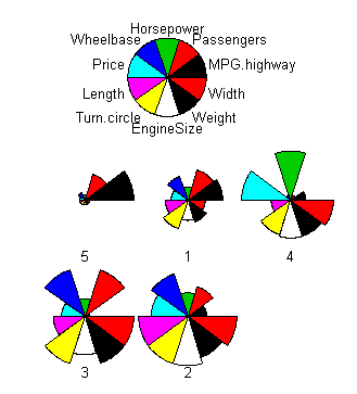
levels(x$cluster) <- c("midsize","luxury","minivan","sporty","compact")
You can also make a star plot of the cars themselves (figure omitted):
x$cluster <- NULL
star.plot(x)
Notice that the rows have been reordered in the star plot so that similar stars are close together. This is makes it a lot easier to read the plot, especially when there are lots of stars. How does star.plot do this? The trick is to use PCA projection. By projecting the multivariate data onto one dimension, we automatically get an ordering in which similar points are close together. star.plot sorts the points according to their 1D PCA projection. It also uses the coefficients of the projection to sort the variables, so that correlated variables are close together on the circle.
Most packages use what I call the "box" scaling, where each variable is scaled to the range [0,1]. Here is what it looks like on the car clusters:
parallel.plot(x,type="box")
An alternative approach is to scale the variables in such a way that the profiles are as linear as possible. Mathematically, we want the approximate equation
xij*sj = ai + bi*vjwhere xij is the data, sj is the scale of variable j, (bi,ai) is the slope and intercept of the line for row i, and vj is the horizontal position of variable j. The best choice of (s,a,b,v) is found by singular value decomposition. When we scale the variables by sj and position them according to vj, we get the following plot:
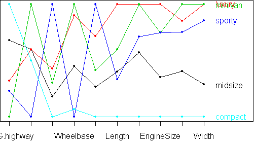
parallel.plot(x)
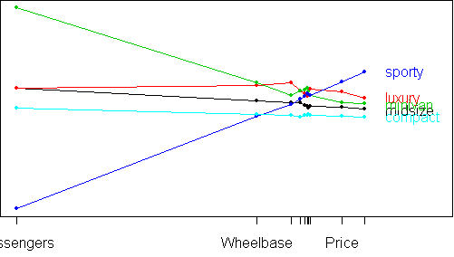
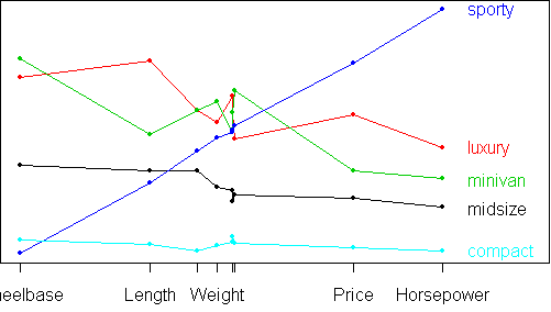
From this plot, a great deal of structure is revealed. As you move from compact to midsize to luxury and minivan, all car attributes increase, except for the number of passengers which doesn't change between midsize and luxury but changes greatly for minivans. Sporty cars buck this trend: they have the highest values for price and horsepower, yet the smallest number of passengers. They have the turn.circle of a midsize, yet the wheelbase of a compact. To get more detail, we can remove the Passengers variable:
parallel.plot(not(x,"Passengers"))
sx <- scale(x)
hc <- hclust(dist(sx)^2,method="ward")
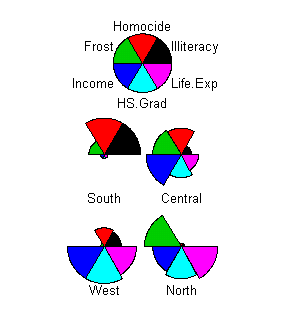
x$cluster <- factor(cutree(hc,k=4))
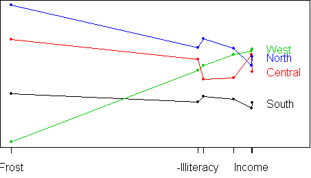
levels(x$cluster) <- c("South","Central","West","North")
star.plot(x)
parallel.plot(x)