To give an example of sensitivity (some would call it fragility), look at the mtcars example on day19. Three predictors, disp, hp, and wt, were equally good to use as the first split. But due to tiny variations in the data, wt was chosen as the split. If we sampled a different set of cars, or left some out, we could easily get a different split and thus a different tree. The predictions would probably be similar, but the interpretation of the predictions would be different.
If a model can only give coarse predictions, is it of any use in data mining? Yes, because we can use it to look deeper into the data. This is done by examining the prediction errors of the model (residuals), which can be quite informative. The coarse model found by a decision tree represents the dominant factors influencing the response. Typically these factors are so obvious that they are not interesting from a data mining perspective. But deviations from the dominant trends, the second-order effects, are often interesting and actionable.
               Type Price MPG.city MPG.highway AirBags DriveTrain Cylinders EngineSize
Acura Integra Small  15.9       25          31    None      Front         4        1.8
              Horsepower  RPM Rev.per.mile Man.trans.avail Fuel.tank.capacity Passengers
Acura Integra        140 6300         2890             Yes               13.2          5
              Length Wheelbase Width Turn.circle Rear.seat.room Luggage.room Weight  Origin
Acura Integra    177       102    68          37           26.5           11   2705 non-USA
We want to predict Price from the other characteristics, some of which are
categorical and some numerical.
We can only guess at the cause-and-effect
of prices, but basically we want some idea of what characteristics are most
valuable in a car.
(Cars are sold at varying prices, depending on the option package. These are
midrange prices.)
Our first result is the following tree:
> tree(Price~.,Cars93)
node), split, n, yval
      * denotes terminal node

 1) root 93 8584.00 19.51
   2) Horsepower < 171 73 2491.00 16.05
     4) Weight < 2742.5 29  129.40 10.84 *
     5) Weight > 2742.5 44 1054.00 19.49
      10) MPG.city < 21.5 30  765.10 21.00
        20) AirBags: None 10   44.74 17.50 *
        21) AirBags: Driver & Passenger,Driver only 20  536.90 22.74
          42) Width < 73.5 13  366.10 24.54 *
          43) Width > 73.5 7   51.39 19.41 *
      11) MPG.city > 21.5 14   73.93 16.25 *
   3) Horsepower > 171 20 2032.00 32.13
     6) Horsepower < 215.5 13  504.60 27.79 *
     7) Horsepower > 215.5 7  826.70 40.20 *
To make a partition plot, we need to focus on two variables. Here Horsepower
and Weight are dominant:
tr <- tree(Price~Horsepower+Weight,Cars93)
cplot(tr)
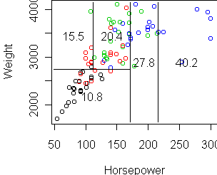
> predict(tr,Cars93)
Acura Integra             Acura Legend                  Audi 90
         10.8                     27.8                     27.8
     Audi 100                 BMW 535i            Buick Century
         27.8                     27.8                     15.5
To see the prediction errors, we can subtract these from the true prices,
or equivalently call the residuals function:
> Cars93$Price - predict(tr,Cars93)
> residuals(tr)
Acura Integra             Acura Legend                  Audi 90
         5.06                     6.11                     1.31
     Audi 100                 BMW 535i            Buick Century
         9.91                     2.21                     0.22
These residuals are in units of $1,000. Sorting the residuals shows the
"overpriced" versus "bargain" cars, at least according to the crude
Horsepower/Weight predictions made by the above tree.
To get at the second-order effects, we model the residuals. Make a copy of the original data frame and change Price to the residual prices. Then fit a tree.
> x <- Cars93
> x$Price <- residuals(tr)
> tree(Price ~., x)
node), split, n, deviance, yval
      * denotes terminal node

 1) root  93 -3e-015
   2) Wheelbase < 104.5  53 -1
     4) Weight < 2780  30 0.3
       8) Horsepower < 83.5   9 -2 *
       9) Horsepower > 83.5  21 1
        18) Weight < 2630  15 0.5 *
        19) Weight > 2630   6 4 *
     5) Weight > 2780  23 -3
      10) RPM < 5700  16 -2 *
      11) RPM > 5700   7 -6 *
   3) Wheelbase > 104.5  40 2
     6) Turn.circle < 38.5   7 8 *
     7) Turn.circle > 38.5  33 0.2
      14) Length < 196.5  18 -1
        28) AirBags: None   6 -3 *
        29) AirBags: Driver & Passenger,Driver only  12 -0.2 *
      15) Length > 196.5  15 2
        30) Width < 73.5   6 7 *
        31) Width > 73.5   9 -2 *
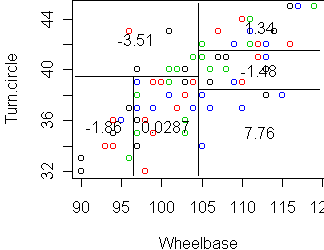
Node 6 has a large mean residual (8). This node is determined by Wheelbase
and Turn.circle, so let's focus on those two variables.
tr2 <- tree(Price ~ Wheelbase+Turn.circle, x)
cplot(tr2)