The idea behind recursive partitioning is to repeatedly select the most relevant predictor variable and use it to stratify the data. Within each stratum, we select the most relevant predictor on that data and sub-stratify until the strata are so small that we run out of data. The result is a stratification tree. By design, the responses within each stratum are as similar as possible. The usefulness of this procedure for data mining is that it finds the main subdivisions of the data as well as the most relevant predictors. It is not particularly good at providing a model for the data or making detailed predictions.
When predictors are categorical, there are different ways to implement this scheme. One way is to stratify across all values of the predictor. Another way, which works better, is to abstract the predictor into two values and stratify only across those two.
The relevance of a predictor is measured either by the sum of squares criterion or the sum of log-variance criterion, depending on your assumptions about the response variance. After abstraction into two bins, the predictor which has smallest sum of squares or smallest sum of log-variance is the most relevant.
  Age Gender Residence Rate
50-54 Female     Urban  8.4
60-64 Female     Rural 20.3
50-54   Male     Rural 11.7
55-59   Male     Rural 18.1
70-74 Female     Urban 50.0
...
Using the function break.factor, we can abstract Age into two bins and measure the sum of squares:
> break.factor(x$Age, x$Rate, 2)
sum of squares = 2178.565
[1] "50-54.55-59.60-64" "65-69.70-74"
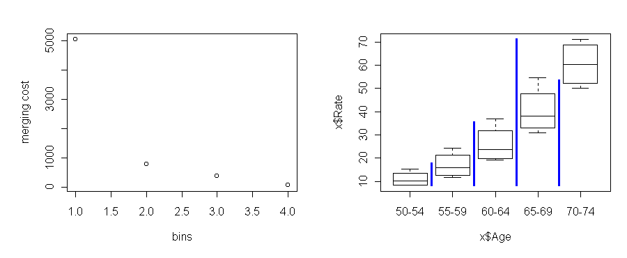
Within the first stratum, ages 50-64, the most relevant variable is still Age. So we stratify Age some more. Within the 60-64 substratum, we find that Gender is now the most relevant predictor. And so on.
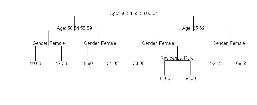
The full tree can be generated with the tree command:
> tr <- tree(Rate ~ ., x, minsize=1)
> tr
node), split, n, yval
      * denotes terminal node

 1) root 20 30.92
   2) Age: 50-54,55-59,60-64 12 17.95
     4) Age: 50-54,55-59  8 13.99
       8) Gender: Female  4 10.60 *
       9) Gender: Male  4 17.38 *
     5) Age: 60-64  4 25.88
      10) Gender: Female  2 19.80 *
      11) Gender: Male  2 31.95 *
   3) Age: 65-69,70-74  8 50.38
     6) Age: 65-69  4 40.40
      12) Gender: Female  2 33.00 *
      13) Gender: Male  2 47.80
        26) Residence: Rural  1 41.00 *
        27) Residence: Urban  1 54.60 *
     7) Age: 70-74  4 60.35
      14) Gender: Female  2 52.15 *
      15) Gender: Male  2 68.55 *
The tree command always uses the sum of squares (same variance)
criterion.
As argued in the analysis above, the first stratification is between ages
50-64 and 65-74. After stratifying on Age, the most relevant
variable in all strata is Gender.
Finally, Residence appears but only in the (Age = 65-69,
Gender = Male) stratum. In other strata, Residence makes
so little impact on Rate that the tree function simply stops
partitioning. The minsize=1 option was necessary
for this dataset because of the way it was represented (only one data row
per predictor combination).
Trees can also be plotted in the following way in S:
plot(tr,type="u");text(tr,pretty=0)
                     Price Country   Type
Volkswagen Fox 4      7225    Brzl  Small
Porsche 944          41990    Grmn Sporty
Chrysler Imperial V6 25495     USA Medium
Buick Electra V6     20225     USA  Large
Ford Probe           11470     USA Sporty
...
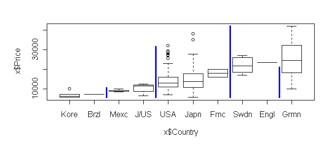
We want to predict Price from the other two categorical variables.
Here are the results of break.factor:> break.factor(x$Country, x$Price, 2) sum of squares = 5876419790 [1] "Kore.Brzl.Mexc.J/US.USA.Japn.Frnc" [2] "Swdn.Engl.Grmn"
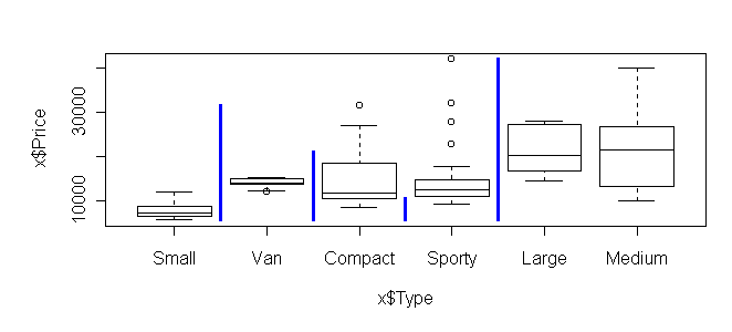
> break.factor(x$Type, x$Price, 2)
sum of squares = 5551739740
[1] "Small.Van.Compact.Sporty" "Large.Medium"
> tr <- tree(Price ~ ., x)
> tr
node), split, n, yval
      * denotes terminal node

 1) root 117 15740
   2) Type: Compact,Small,Sporty,Van  80 13040
     4) Country: Brzl,Frnc,Japn,J/US,Kore,Mexc,USA  69 11560
       8) Type: Small  21  7629 *
       9) Type: Compact,Sporty,Van  48 13270
        18) Country: J/US,Mexc,USA  29 12240 *
        19) Country: Frnc,Japn  19 14850 *
     5) Country: Grmn,Swdn  11 22320 *
   3) Type: Large,Medium  37 21600
     6) Country: Frnc,Kore,USA  25 18700
      12) Type: Large   7 21500 *
      13) Type: Medium  18 17610 *
     7) Country: Engl,Grmn,Japn,Swdn  12 27650 *
To get a list of the cases that fall into a particular stratum, use the
function cases.tree. For example, suppose we want the cars
under node 4:
> cases.tree(tr,"4")
 [1]   1   2   3   4   5   6   7   8   9  10  11  12  13  14
[15]  15  16  17  18  19  20  21  23  24  25  26  27  28  29
[29]  30  31  32  33  34  35  36  37  38  39  40  41  42  44
[43]  45  46  48  52  53  54  55  56  57  58  59  61  62  63
[57]  64  65  68  69 108 109 110 111 112 113 114 115 116
> y <- x[cases.tree(tr,"4"),]
y is now a reduced table containing only those cars. If we run break.factor on y, we find that Type is the most relevant predictor, which confirms the split made at node 4 into Type = Small versus Compact,Sporty,Van.
Consider this dataset from Motor Trend magazine describing characteristics of 32 cars:
                   mpg cyl disp  hp drat    wt  qsec vs am gear carb
Mazda RX4         21.0   6  160 110 3.90 2.620 16.46  0  1    4    4
Mazda RX4 Wag     21.0   6  160 110 3.90 2.875 17.02  0  1    4    4
Datsun 710        22.8   4  108  93 3.85 2.320 18.61  1  1    4    1
Hornet 4 Drive    21.4   6  258 110 3.08 3.215 19.44  1  0    3    1
Hornet Sportabout 18.7   8  360 175 3.15 3.440 17.02  0  0    3    2
...
We want to predict mpg (fuel efficiency) from the other predictors, which
include engine displacement, rear axle ratio, number of forward gears, etc.
A first-cut visualization of the data can be obtained by plotting mpg
against each predictor individually: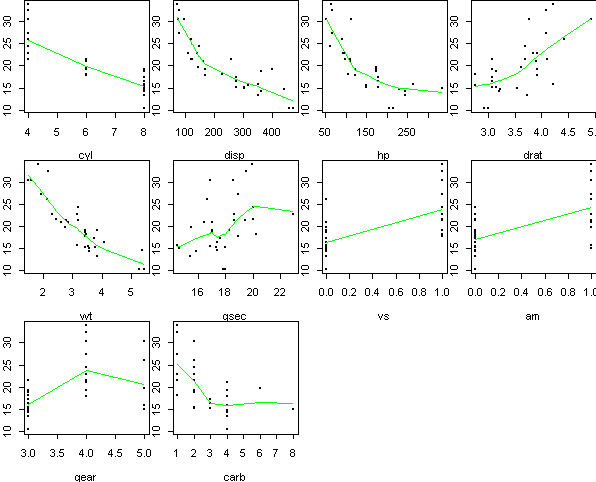
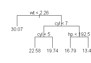
> tr <- tree(mpg ~ ., mtcars)
> tr
node), split, n, yval
      * denotes terminal node

 1) root 32 20.09
   2) wt < 2.26  6 30.07 *
   3) wt > 2.26 26 17.79
     6) cyl < 7 12 20.93
      12) cyl < 5  5 22.58 *
      13) cyl > 5  7 19.74 *
     7) cyl > 7 14 15.1
      14) hp < 192.5  7 16.79 *
      15) hp > 192.5  7 13.41 *
> plot(tr,type="uniform"); text(tr,pretty=0)
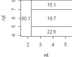
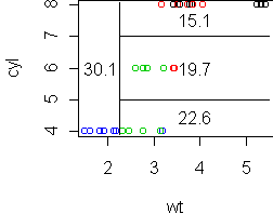
tr <- tree(mpg ~ wt+cyl, mtcars)
partition.tree(tr)
cplot(tr)
Functions used in this lecture: