A Standard Custom Interface for Common sklearn Classification Models
Background, initial motivation, and development data set
I wanted to apply to classification models the same methodology I used to create a customized interface for heatmap plots . Similarly to the creation of heatmaps, the process of instantiating and training models tends to use the same steps (with some modifications) over and over, and after training there is a similarly stereotyped set of things one tends to do with the model. The big difference is that instead of a one-time-use function for outputting a plot, it made more sense to me to implement these classifiers as custom Python objects—each essentially a wrapper for a particular scikit-learn classifier, with a more streamlined initiation procedure and some convenient methods added. For development purposes I intially focused on the RandomForestClassifier from sklearn.ensemble.
The MNIST data set of images of handwritten digits is a benchmark for a basic classification algorithm. It consists of 60,000 training images and 10,000 test images, each of a handwritten digit from 0 to 9. Here are the first three hundred thirty-six images in the training set, stitched together for display:
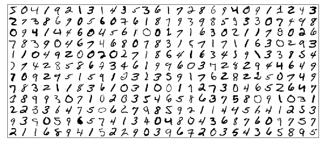
Each image is 28x28 pixels, and is encoded as an array of grayscale values ranging from 0 (white) to 255 (black) for each pixel. These properties of the data set allow it to serve as a paradigmatic example of a broad type of machine learning classification problem: given an input data point with a potentially very large number of numerical variables, output a single categorical label, chosen from one of a relatively small number of possibilities. For these data, a functional model will have 'learned', based on the training set, patterns of relationships among the seven hundred eighty-four pixel values that allow it to choose the most likely digit to assign to a given test image.
Data Preparation
In principle, a classifier can be trained on a data set with any number of scalar columns containing numerical values, and exactly one category column indicating class membership. Similarly to the behavior of my custom heatmap interface, calling the classifier requires a dataframe input, and allows for optional
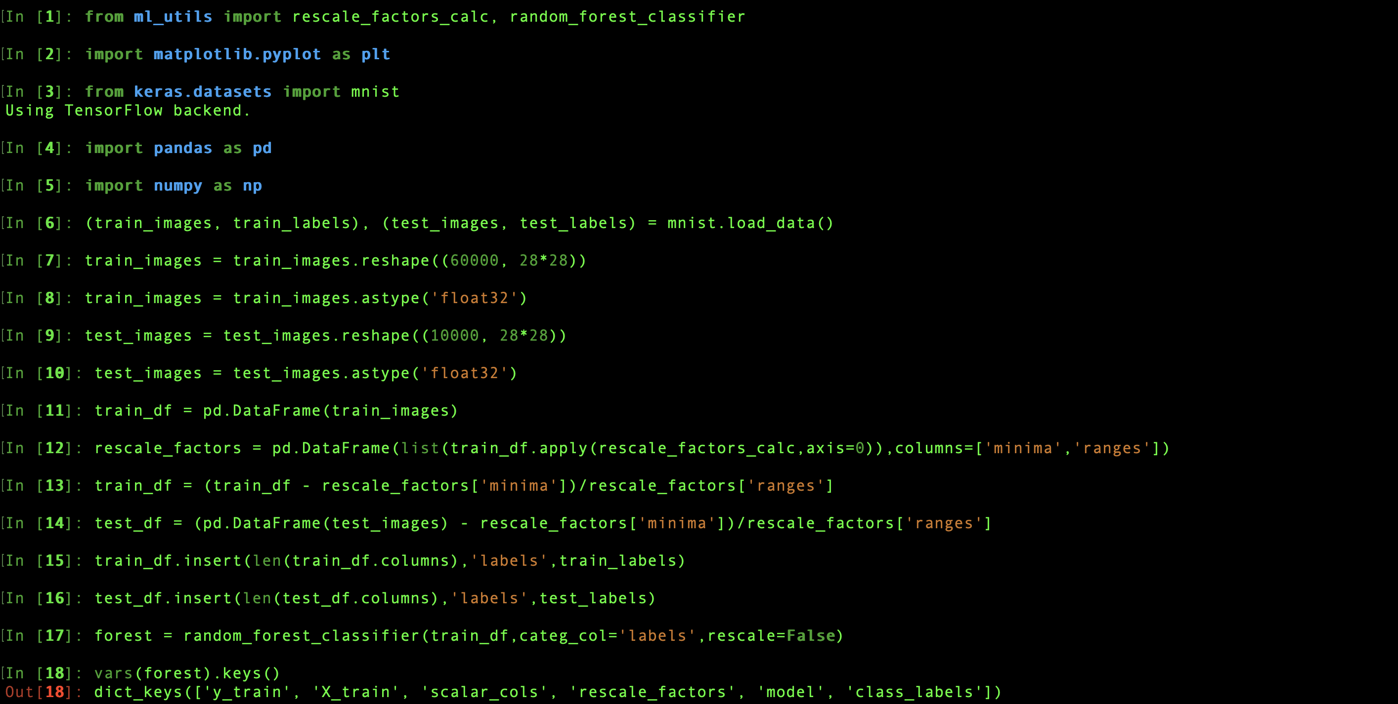
In practice, for algorithm performance it's often necessary to condition the data to make sure that there aren't columns with a signficantly greater or smaller magnitude of values than the others (this is more likely to be an issue when combining columns that have different units and different inherent numerical ranges unlike this pixel data, but it's important to keep in mind). The default behavior is to independently rescale each column by finding its minimum and maximum values in the training data, subtracting the minimum from each value in the column, and dividing each value by the range between maximum and minimum, thus forcing each column to range between 0 and 1. For this example, I've explictly shown the same operations the classifer would normally be capable of doing invisibly. This behavior can be suppressed when initializing the classifier by setting the
Initial classifier attributes and methods
The rescale values for each column are saved in an attribute of the classifier, classifier.rescale_factors, so that when a new data set is fed to it, each column will be rescaled with the same parameters as the training set. The set of scalar input column names (classifier.scalar_cols) and the list of possible class labels (classifier.class_labels) are also saved. The column names must all be present in any test data so they can be fed into the model, and the class labels are used to determine the possible range of predictions. The training data and labels used to create the classifier are likewise stored in classifier.X_train and classifier.y_train, while the underlying trained sklearn model can be accessed as classifier.model.
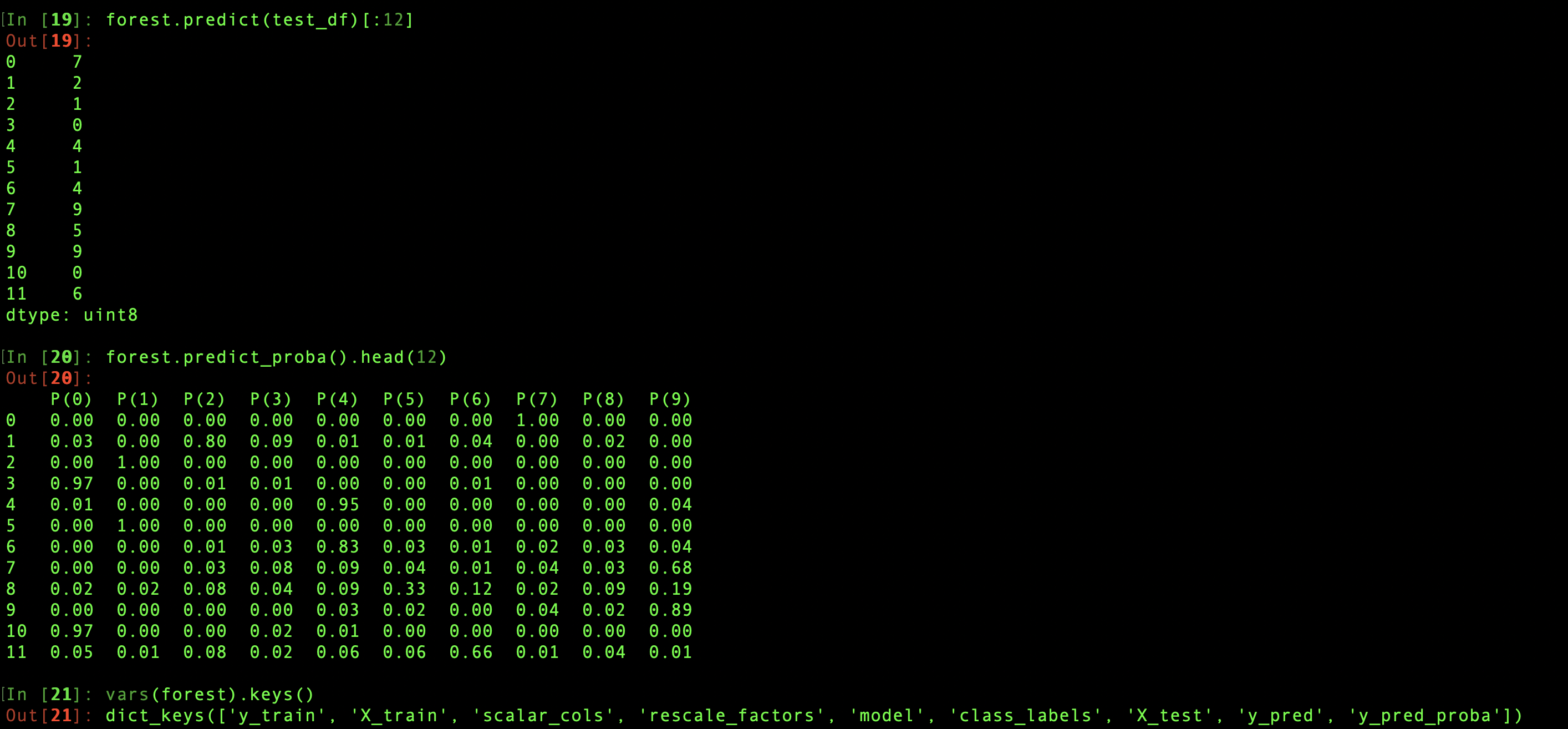
Each classifier object also comes with nine explicitly defined methods that interact with this set of attributes and may modify them or create others. The classifier.predict method takes a dataframe of test data as its argument and uses the trained model to return a series of of the most likely label for each data point. When predict is called, the test set and the predictions are saved as attributes of the classifier, classifier.X_test and classifier.y_pred. If the method is called without an argument, it uses the saved value of X_test as input.
The classifier.predict_proba method has similar behavior. It returns a dataframe showing the probability of assigning each of the possible class labels to each of the test data points, and stores that result in classifier.y_pred_proba. Then classifier.y_pred is updated based on these probabilities—each test data image is assigned the label with the highest probability—to make sure these two attributes both agree with the last input and each other. For the same reason, if predict is called directly after y_pred_proba has been defined, the attribute will be deleted, since it's now obsolete.
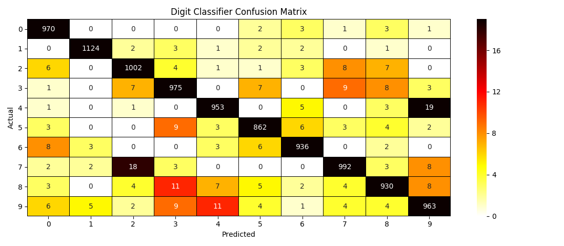
Confusion matrices
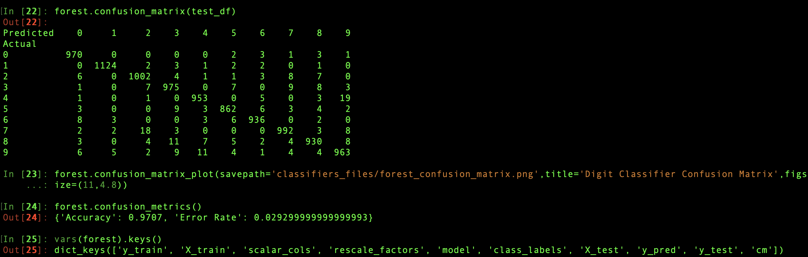
There are three methods that calculate a test data set's confusion matrix, the grid of counts of actual class assignments for each predicted assignment. Each saves the result as a dataframe in classifier.cm, and each will retrieve the confusion matrix from this attribute if called without input test data. If test data is supplied, it must include, either as a column of the test dataframe with the same name as classifier.y_train or as a separate input parameter, the true categories, which are then stored as classifer.y_test. Then classifier.predict is called with the test dataframe, updating classifier.X_test and classifier.y_pred in the process. It's after constructing the confusion matrix from y_test and y_pred that the three methods behave differently.
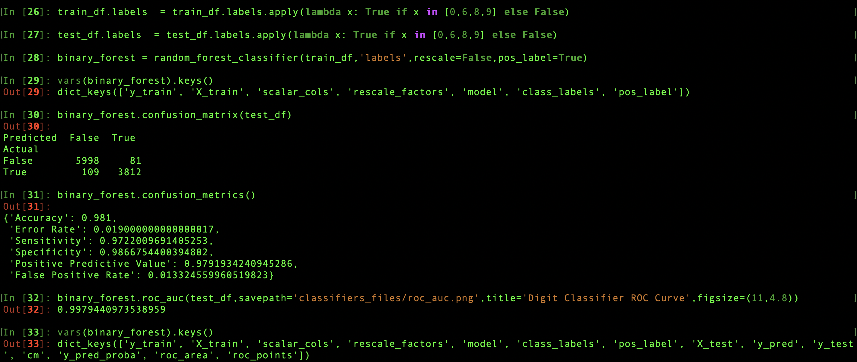
classifier.confusion_matrix simply returns the dataframe, while classifier.confusion_matrix_plot returns nothing, but automatically creates a heatmap plot from the matrix. A filepath can be provided to save the image, or, in the absence of this savepath, plt.show is called. Finally, classifier.confusion_metrics calculates the test accuracy from the sum of the on-diagonal elements of the matrix, divided by the total sum, and the error rate by subtracting the accuracy from 1. These two metrics are returned together as a dictionary, though not saved, since they can be so easily recalculated from classifier.cm
Binary classifiers
Binary classifiers, those with only two class labels, have some slightly different behavior with respect to classifier.confusion_metrics. First of all, when a classifier is initiated using a data set with only two classes, a classifier.pos_label attribute is created. The category label to consider positive can be specified by the user, or it will be automatically chosen to be the second label found in the training category column. The positive label assignment is needed for the calculations specific to binary classifiers. These include four additional metrics—sensitivity, specificity, positive predictive value, and false positive rate—that are derived from the 2x2 confusion matrix and returned along with the accuracy and error rate.
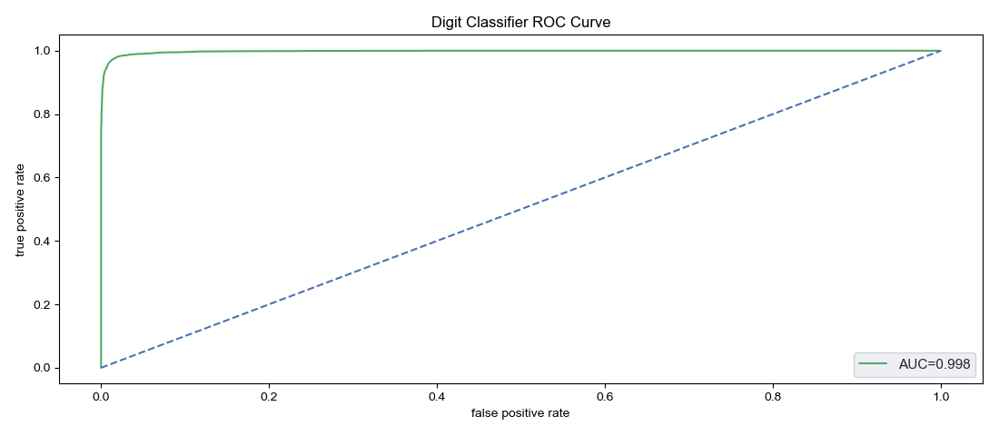
The classifier.roc_auc method calculates and returns the receiver operating characteristic (ROC) area under the curve. The ROC curve plots sensitivity against false positive rate for varying probability thresholds, so classifer.predict_proba is internally called on the supplied test data set, creating or updating the usual attributes discussed above. At the same time, a plot of the ROC curve is generated and returned, either saving as an image to a specified destination savepath, or being presented via plt.show. The area is saved in the attribute classifier.roc_area, while the calculated points on the curve used for the plot are saved as a dataframe, classifier.roc_points. This dataframe actually has three columns: roc_points.fpr and roc_points.tpr are the horizontal and vertical coordinates for each point on the curve, while roc_points.threshold are the probability thresholds for which each pair of false positive rate and true positive rate was calculated. If called without a test data set, classifier.roc_auc doesn't make any calculations, but returns the saved classifier.roc_area and uses the saved classifier.roc_points to make a plot. The method is available only for binary classifiers; if there are anything other than two classes the method will return nothing and do nothing.
Saving and recalling a classifier
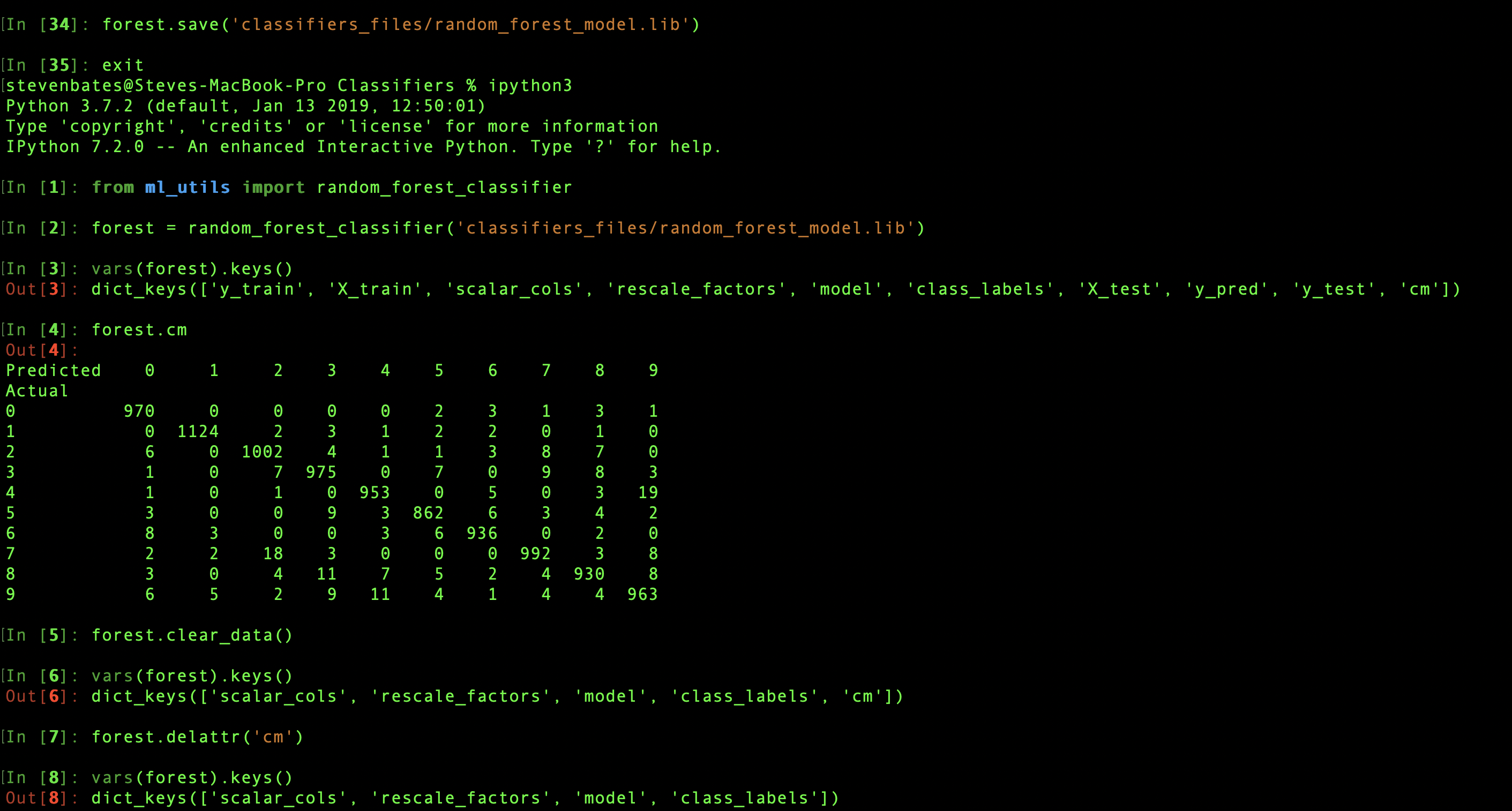
To take advantage of the portability gained by wrapping all the data and metrics associated with a model in a single object, I also added a save method, which leverages the joblib library. The method takes a destination filepath as the argument. After saving, a classifier can be recalled later in a new environment by calling random_forest_classifier. When the argument is a string instead of a dataset, the initialization routine knows to interpret that as a filepath and reload the saved classifier.
Because training and test data will likely have been saved separately, it may not be desirable for them to needlessly take up space by also being saved as part of the classifier. For convenience, the classifier.clear_data method will remove classifer.X_train, classifier.y_train, classier.X_test, classifier.y_test, classifier.y_pred, and classifier.y_pred_proba. Any attribute can also be removed individually by name using the classifer.del_attr method.
Conclusion and other notes
After going through it once with sklearn.ensemble.RandomForestClassifier, it was easy to apply the same procedure to create a wrapper for sklearn.linear_model.LogisticRegression, sklearn.ensemble.GradientBoostingClassifier, sklearn.svm.LinearSVC/sklearn.svm.SVC, and sklearn.linear_model.RidgeClassifier. As with random_forest_classifier, these classes—log_reg_classifier, grad_boost_classifier, svm_classifier, and ridge_reg_classifier—take training data as a mandatory argument when called, but also have optional arguments and defaults which correspond to each of the parameters explicitly listed in the docstring of the sklearn models, to which they are passed, as well as the fit method of the model along with the training data. This interface will therefore make it easy to loop through many model iterations comparing performance as parameters are systematically changed within the same model type, as well as across multiple types.
The svm_classifier has a special Boolean sklearn.svm.LinearSVC or sklearn.svm.SVC as the model. The differences are explained in more detail in the scikit-learn documentation, but the upshot is that the linear version allows only hyperplanes as boundaries for the hyperspace regions corresponding to each category, while the general model allows for arbitrary boundary shapes. This means the latter is significantly more data intensive than the former, taking over seventy minutes to train with the MNIST set on my Macbook Pro with all other settings default. Of the others, only grad_boost_classifier takes anywhere close to as long, at around twenty-two minutes. The others, including svm_classifier with
Neither sklearn.linear_model.RidgeClassifier nor sklearn.svm.LinearSVC has a predict_proba method, so ridge_reg_classifier has its predict_proba method removed as well, while calling predict_proba on an svm_classifier using a linear model will raise an error. Since the roc_auc method is no longer able to leverage predict_proba to generate the ROC curve, in these special cases the decision_function method of the sklearn model is called instead, generating confidence scores that play the thresholding role that would otherwise have been filled by prediction probabilities in the ROC calculation process.
Links
ml_utils library including these and other useful objects and methods on github
A pared down version of the previous, with only classifiers
Documentation for each of the underlying sklearn classifiers: random forest, gradient boosted decision trees, logistic regression, ridge regression, linear support vector machine, general support vector machine
An overview of the random forest algorithm
An explanation of the math behind logistic regression