Day 32 - Applying logistic regression
Today we look at practical aspects of using logistic regression for
classification, and how it
compares to the other classification methods in this course.
Spam filtering
Unsolicited bulk email, aka spam, is an annoyance for many
people. Suppose you wanted to make a classifier to detect spam and filter
it out of your mail. How would you do it? There are four basic steps:
- Collect a dataset of email labeled as "spam" and "not spam".
- Define variables which can be used to discriminate the two classes.
This is sometimes called feature extraction.
- Divide the data into a training set and test set.
- Train a classifier and evaluate it on the test set.
In this course, we have described three methods for classification:
- histograms
- trees
- logistic regression
We'll use the spam example to compare their properties.
George Forman, a researcher at Hewlett-Packard, has made a spam
dataset.
He took 4601 of his own email messages, labeled them,
and extracted various features.
The features include the frequency of various words (e.g. "money"),
special characters (e.g. dollar signs), and the use of capital letters
in the message.
For each message, the following variables are recorded:
> colnames(x)
 [1] "word.freq.make"
 [2] "word.freq.address"
 [3] "word.freq.all"
 [4] "word.freq.3d"
    ...
[48] "word.freq.conference"
[49] "char.freq.semi"
[50] "char.freq.paren"
[51] "char.freq.bracket"
[52] "char.freq.bang"
[53] "char.freq.dollar"
[54] "char.freq.pound"
[55] "capital.run.length.average"
[56] "capital.run.length.longest"
[57] "capital.run.length.total"
[58] "spam"
The last variable is the class variable ("Yes" or "No").
These variables only describe the content of the message.
In a real system, we would probably also want to compare the sender name to
an address book.
We split into train and test:
x <- rsplit(x,0.5); names(x) <- c("train","test")
For a tree classifier, these are the commands we would use:
tr <- tree(spam~.,x$train)
plot(tr,type="u");text(tr,pretty=0)
The resulting tree depends strongly
on the particular train/test split. Some variables which appear
consistently are the frequency of dollar signs, exclamation points, and the
word "hp", which is a good indicator of non-spam in this dataset.
The tree is rather complicated, but only uses a few variables.
Trees tend to use only a few variables, which is great for analysis but not
so good for classification. For good classifications we should want to use
as much information about the message as possible.
Logistic regression is quite different from trees in that it uses
all of the variables.
We can make a logistic regression classifier as follows:
fit <- glm(spam~.,x$train,family=binomial)
The error rate for both models can be computed using misclass:
> misclass(tr,x$test)
[1] 224
> misclass(fit,x$test)
[1] 168
For one particular train/test split, the tree has 224/2300 errors while
logistic regression has 168/2300.
This difference is statistically
significant:
> chisq.test(array(c(224,2300,168,2300),c(2,2)))
X-squared = 7.0897, df = 1, p-value = 0.007753
Cross-validation on tree size does not change the error rate.
Misclassification rate is not an entirely appropriate measure for this
problem, because the costs are not equal.
I would say that C(y|n) (falsely classifying as spam)
is greater than C(n|y).
We can get a better idea of
performance by making a confusion matrix:
> confusion(tr,x$test)
     predicted
truth   No Yes
  No  1330  82
  Yes  142 746
> confusion(fit,x$test)
     predicted
truth   No Yes
  No  1345  67
  Yes  101 787
Logistic regression makes less errors of both type, so it is a better
classifier for this data no matter what the cost structure.
Can a tree ever be better than logistic regression? Absolutely. Remember
that logistic regression always uses a linear boundary between the classes.
But trees are not so constrained: a big enough tree, with small enough
cells, can represent any class boundary. The problem is having enough data
to figure out what that boundary is. If the tree doesn't have enough data,
it will use a boundary with lots of corners. Therefore logistic regression
wins in the above example because the true boundary is close to linear and
the training set isn't big enough for the tree to figure this out.
Histogram method
What about the histogram method that we introduced on day3? It can also be used to classify text documents.
In fact, it has a lot in common with logistic regression. Both are
linear classifiers, in the sense that they take a linear
function of the predictors and compare it to zero. For logistic
regression, we look at whether p(y=1|x) > 0.5, which is
equivalent to a + b*x > 0. In the histogram method, we look at
whether L(pop1) > L(pop2), where
L(pop) = sum_w n_w log p(w | pop). But this is equivalent to
sum_w n_w b_w > 0, where the word coefficient b_w = log p(w
| pop1)/p(w | pop2).
Linear classifiers have been used since the early days of computing, since
they are so easy to implement in hardware. In theory, you just need a few
potentiometers to represent the coefficients. At the time, they were
called neural networks, by analogy to how neurons in the brain
combine messages from their neighbors (perhaps linearly) and then decide to
"fire" or "not fire" (perhaps by thresholding at zero). Since then, a
variety of spinoff methods have been developed, which were also called
neural networks. Eventually it got to a point where every new
classification algorithm was called a neural network. Consequently the
term carries little information today.
So what's the difference between logistic regression and the histogram
method? For one thing, the histogram method has a very specific idea of
what the predictors are. It regards each document as a batch of
independent observations; the predictors are relative frequencies within
the batch. The predictors must refer to disjoint possibilities. For
example, word.freq.make and
capital.run.length.average are not disjoint, because "make"
could be capitalized. To use the histogram method on the spam dataset, we
have to restrict ourselves to the word variables.
Secondly, the histogram method chooses its coefficients differently than
logistic regression. Logistic regression chooses coefficients which
separate the training data as well as possible. The histogram method
tries to model the two classes, based on an independence assumption.
This constraint means that the histogram method can only achieve a subset
of the possible linear classifiers. But as we saw above, constraints
aren't necessarily bad.
To test this theory, a logistic regression classifier (fit) and
a histogram classifier (fit2) were trained on the spam dataset
using word variables only.
Here are the results:
> misclass(fit,x$test)
[1] 216
> misclass(fit2,x$test)
[1] 309
This is the same train/test split used above, so we see that restricting to
word variables has worsened the logistic regression to 216/2300 errors.
The histogram classifier, even though it is also a linear classifier, does
significantly worse.
Here's what happens if we do the same thing, but with the training set
reduced to 231 examples:
> misclass(fit,x$train)
[1] 2
> misclass(fit2,x$train)
[1] 34
> misclass(fit,x$test)
[1] 755
> misclass(fit2,x$test)
[1] 564
Logistic regression does much better on the training set, as expected, but
worse on the test set.
How can this be? Logistic regression could easily have found the same linear
classifier as the histogram method. But it chose another classifier which
seemed better on the training set.
The additional constraint imposed by the histogram
method has helped it find a better classifier when the amount of data is
small.
Learning theory
Numerous studies in machine learning have shown that this sort of behavior
is typical: more constrained classifiers do better on small datasets.
But does this mean that constraints are good? If so, which ones?
Many machine learning researchers have pondered this question, and the
answer remains controversial. Some say that any constraint can be
used, and the game is simply to tune the amount of constraint to the amount
of data. As a theory of learning, this seems too crude.
Bayesian statistics provides a better explanation.
According to Bayesian statistics, most classifiers, including logistic
regression and trees, are using the wrong criteria to learn from a training
set. For example, let's look at the criterion used by logistic regression.
This is the maximum-likelihood formula given on day31. Look at what happens when the classes are
perfectly separable:
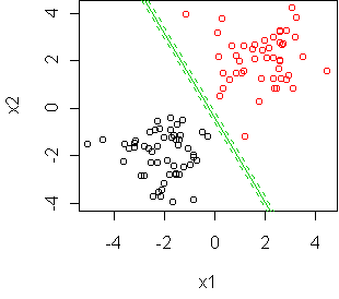
In such cases, it can be
shown that maximum-likelihood will try to place the boundary as far away
from the data as possible. Specifically, it will maximize the
margin: the distance to the closest boundary point. A consequence
is that the logistic regression coefficients are determined completely by
the boundary points (three points, in this case).
Some people say this is a good thing, because it makes the estimates robust
to noise in most of the dataset. On the other hand, it is bad, because it
throws away information in the dataset and makes the estimate very
sensitive to the position of the boundary points. Consider this example:
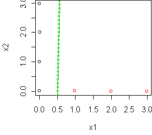
The maximum-margin solution is a vertical
line, determined only by the two points at (0,0) and (1,0). (The line is
not perfectly vertical in the figure because the optimization was stopped
early. glm has problems with separated classes.) By moving
those two points, we can swing the estimated boundary all the way from
vertical to nearly horizontal:
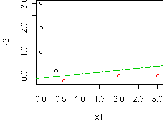
A better option in these situations is to consider all of the possible
classifiers, not just the one which has some special geometrical property.
For the above example, the classifiers range from vertical (90 degrees) to
horizontal (0 degrees). To hedge our bets among them, we should pick the
average: 45 degrees. Note that this is similar to what we would get if we
used bagging on logistic regression: by taking random subsets of the
training data, the boundary would swing from 0 to 90 degrees, and when we
voted them we would be classifying according to the 45 degree line.
According to Bayesian statistics, you should always average when
making predictions. So I am recommending a Bayesian approach to linear
classification. For my PhD thesis, I developed a technique for efficiently
computing the average linear classifier. It outperforms
logistic regression on many real-world datasets, which adds support for the
theory.
Another problem with maximum-likelihood logistic regression is that it will
always choose a classifier which separates the data, if this is possible.
Along with maximum-margin, this is what causes logistic regression to
overfit. A proper criterion would allow logistic regression to make errors
on the training set, even if it didn't have to. We can achieve this by
enlarging the averaging process to include classifiers that make errors.
So what about constrained classifiers? By the above arguments, constrained
classifiers succeed because their constraints bring them close to the
average classifier, when the training set is small. Hence some constraints
really are better than others.
Code
Functions introduced in this lecture:
References
The paper "Discriminative
vs Informative Learning" discusses
the pros and cons of modeling the classes (as in the histogram method)
versus separating them (as in logistic regression).
My PhD thesis on
Bayesian linear classifiers and general algorithms for
Bayesian inference. See Chapter 5.
Tom Minka
Last modified: Tue Apr 25 09:48:24 GMT 2006