Day 29 - Multiple regression
Last time we discussed linear regression with one predictor. Now we
consider multiple predictors. We will assume that the predictors are
additive and each has a linear relationship with the response.
Mathematically, this means that y = a + b1*x1 + b2*x2 + ....
We have one slope coefficient for each numerical predictor.
Visualization is more difficult when there are multiple predictors. Our
technique will be to use pairwise scatterplots and residual scatterplots.
There are also inference methods which allow us to quickly determine which
are the relevant and irrelevant predictors.
CMU buildings
A student in the class, Stephen Piercy, has collected and shared with us
a dataset describing
the power consumption of various buildings on the CMU campus.
His interest is in influencing university policy to make our buildings more
efficient.
Here are the first few rows:
                      building.type  sq.ft kwh.elec mlbs.steam mcf.gas kwh.sq.ft lbs.sq.ft cf.sq.ft
Apartments, Houses        Residence 114320   598552         NA    1093      5.24        NA     0.95
407-409 Craig Street Administrative  10118   247560         NA      95     24.47        NA     0.93
6555 Penn Ave        Administrative  99369   538120         NA    3668      5.42        NA     3.69
Alumni Hall          Administrative   8223   107446        783      37     13.07      9.52     0.44
Baker/Porter               Academic 227617  2842770      21778      NA     12.49      9.56       NA
...
We can learn a lot about this dataset just by looking at pairs.
Let's start with electricity consumption (kwh.elec) versus
building size (sq.ft):
predict.plot(kwh.elec~sq.ft, x)

We get the expected result that bigger buildings consume more electricity.
To get more detail, we can apply the bulge rule to transform these
variables.
A log transformation on both variables seems good:
predict.plot(log(kwh.elec)~log(sq.ft), x)
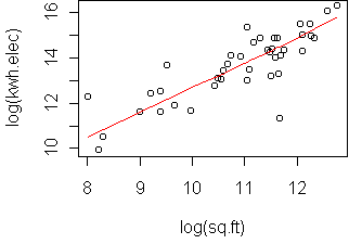
The relationship is quite linear in the log domain.
The least-squares fit is
> lm(log(kwh.elec)~log(sq.ft), x)

Coefficients:
(Intercept)   log(sq.ft)
      2.808        0.993
Taking the slope as 1, this means that
kwh.elec = sq.ft*exp(2.808), or that the ratio
kwh.elec/sq.ft is approximately 16.6 across campus.
Energy efficiency
The variable kwh.sq.ft is defined to be this "energy efficiency"
ratio kwh.elec/sq.ft.
Buildings which deviate from this number are the interesting cases.
So let's try to regress it on the other variables.
We can plot multiple pairs at once using the command
predict.plot(kwh.sq.ft ~ ., x)
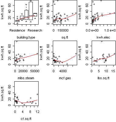
From this we see that many variables correlate with the energy efficiency.
For example, the "steam efficiency" lbs.sq.ft:
predict.plot(kwh.sq.ft~lbs.sq.ft,x)
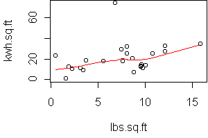
> fit <- lm(kwh.sq.ft~lbs.sq.ft,x)
> fit

Call:
lm(formula = kwh.sq.ft ~ lbs.sq.ft, data = x)

Coefficients:
(Intercept)    lbs.sq.ft
     12.074        1.084
The slope is 1, which is interesting since it implies that energy
efficiency moves together with steam efficiency.
However, there is a fair bit of noise off of the line; how can we be sure
that this effect is real? One approach is to test against the null
hypothesis that the slope is zero. The result of this test can be found in
the output of summary(fit):
> summary(fit)

Call:
lm(formula = kwh.sq.ft ~ lbs.sq.ft, data = x)

Residuals:
    Min      1Q  Median      3Q     Max
-14.807  -9.328  -2.106   4.565  55.095

Coefficients:
            Estimate Std. Error t value Pr(>|t|)
(Intercept)  12.0740     6.2727   1.925   0.0667 .
lbs.sq.ft     1.0845     0.7494   1.447   0.1614
---
Signif. codes:  0 `***' 0.001 `**' 0.01 `*' 0.05 `.' 0.1 ` ' 1

Residual standard error: 14.02 on 23 degrees of freedom
Multiple R-Squared: 0.08345,    Adjusted R-squared: 0.0436
F-statistic: 2.094 on 1 and 23 DF,  p-value: 0.1614
It says that the estimated slope has a probability 0.16 of occurring under
the null hypothesis, which isn't unlikely enough for us to say with
confidence that the slope is nonzero.
Outliers
However, this test might be unduly influenced by the outlier at the top of
the plot. This outlier makes it look like the data is noisier than it
really is.
We can identify the outlier by
using the identify option to predict.plot:
predict.plot(kwh.sq.ft~lbs.sq.ft,x,identify=T)
Left click to identify, right click to exit.
Clicking on the outlier reveals that it is Cyert Hall, home of Computing
Services at CMU.
It uses quite a lot of electricity relative to its size.
Because we can explain this outlier, we are justified in removing it
and doing a new analysis:
x2 <- x[setdiff(rownames(x),"Cyert Hall"),]
predict.plot(kwh.sq.ft~lbs.sq.ft,x2)
fit <- lm(kwh.sq.ft~lbs.sq.ft,x2)
summary(fit)
The summary now gives a p-value of 1%, so the relationship between
lbs.sq.ft and kwh.sq.ft is statistically significant.
Tree measurements
Instead of just pairs, we would like to use all of the predictors together.
Let's try this on the following dataset of tree
measurements:
  Girth Height Volume
1   8.3     70   10.3
2   8.6     65   10.3
3   8.8     63   10.2
4  10.5     72   16.4
5  10.7     81   18.8
...
For logging, it is useful to know how much lumber you will get from a tree
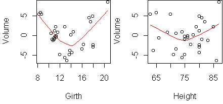
of known girth and height. We start with a predict.plot:
data(trees)
predict.plot(Volume~.,trees)
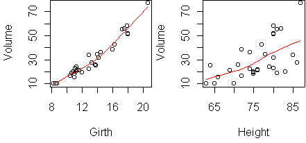
Both variables correlate with Volume. To fit a multiple regression model,
we call lm with both predictors:
> fit <- lm(Volume~.,trees)
> fit <- lm(Volume~Girth+Height,trees)
> fit

Coefficients:
(Intercept)        Girth       Height
   -57.9877       4.7082       0.3393
To see how well we've done, we plot each predictor against the residuals of
the fit. This is done by giving the linear model to predict.plot:
predict.plot(fit)
The residuals have a bulge downwards for each predictor. This suggests
that we transform the response. A log transformation is too much; we are
left
with an upward bulge. A square root is not enough. In fact, the best
transformation is cube root (p=1/3), which we might have guessed from the
units of volume compared to girth and height.
Here is the result:
predict.plot(lm(Volume^(1/3) ~ Height + Girth,trees))
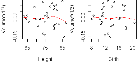
There is no structure left in the residuals, and the R-squared is 97.8%.
From geometry, you might argue that the correct relationship is Volume
= Height*Girth^2. In the log domain, this means log(Volume) =
log(Height) + 2*log(Girth). Let's try this:
> lm(log(Volume) ~ log(Height) + log(Girth),trees)

Coefficients:
(Intercept)  log(Height)   log(Girth)
     -6.632        1.117        1.983
Yes, the geometry seems to be correct.
Interestingly, the R-squared of this fit is
97.8%, the same as above.
Backfitting
To estimate a multiple linear regression model, we minimize the sum of
squares: sum_i (yi - a - b1*xi1 - b2*xi2 - ...)^2. There are
various computational methods to do this minimization. One of them is the
backfitting method described for response tables on day25. If we fix all of the coefficients except one,
then the least-squares problem is the same as simple linear regression for
that one coefficient. If we are estimating b1, then the
responses being fit are the partial residuals (y - a -
b2*x2), and similarly for estimating b2. These are the
same partial residuals that arose in response tables. The backfitting
algorithm is to regress the partial residuals onto each predictor in a
round-robin fashion until the coefficients converge. As in response
tables, this algorithm gives a useful perspective on what the coefficients
mean. They describe the additional effect of the predictor. Coefficient
b1 is the slope of the partial residuals with respect to
x1, which is not necessarily the same as the slope of the
response with respect to x1 that you would see in a
predict.plot
Cement data
Let's try a more complex dataset. This one has four predictors:
  x1 x2 x3 x4     y
1  7 26  6 60  78.5
2  1 29 15 52  74.3
3 11 56  8 20 104.3
4 11 31  8 47  87.6
5  7 52  6 33  95.9
...
The response y is the heat evolved in setting cement, and the
predictors are the proportions of active ingredients in the cement.
The four of them should add to 100 (but usually less due to rounding).
Here is the predict.plot:
predict.plot(y~.,cement)
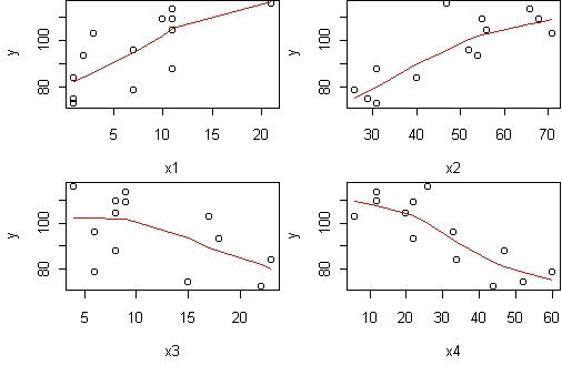
This shows that all predictors are correlated with the response, and that
(x1,x2) are positively related while (x3,x4) are negative.
Let's make a linear fit and see which predictors are relevant:
> fit <- lm(y ~ x1 + x2 + x3 + x4, cement)
> summary(fit)

Coefficients:
            Estimate Std. Error t value Pr(>|t|)
(Intercept)  62.4054    70.0710   0.891   0.3991
x1            1.5511     0.7448   2.083   0.0708 .
x2            0.5102     0.7238   0.705   0.5009
x3            0.1019     0.7547   0.135   0.8959
x4           -0.1441     0.7091  -0.203   0.8441
---
Signif. codes:  0 `***' 0.001 `**' 0.01 `*' 0.05 `.' 0.1 ` ' 1

Residual standard error: 2.446 on 8 degrees of freedom
Multiple R-Squared: 0.9824,     Adjusted R-squared: 0.9736
F-statistic: 111.5 on 4 and 8 DF,  p-value: 4.756e-007
According to this summary, none of the predictors have a statistically
significant effect on the response. How can this be? The
p-value for each predictor assumes that the other predictors are in the
model. The predictors are linearly related by the fact that they sum to
100. Therefore each predictor seems irrelevant when you know the other
three.
This illustrates a danger in trying to interpret p-value summaries.
A more robust way to determine relevant variables is to fit models with
different variables included and see which one is best. In doing this, we
have to be careful about the meaning of "best". If we just look at the
performance on the training data, via R-squared or the sum of squares,
then we will favor the model which includes all of the predictors. Just as
in building a tree, more complex models always win on the training data.
To truly decide among models we have to infer what will happen on future
data. Cross-validation could be used for this, but it is expensive. For
linear regression, learning theory is a practical alternative.
There are various refinements of the theory of linear regression (some of
which I am developing), but basically everyone agrees that more
coefficients allow you to overfit more. So one has to strike a balance
between the fit on the training set (sum of squares) and the number of
coefficients. One criterion which embodies this tradeoff is the AIC:
(p is the number of coefficients)
AIC = (sum of squares) + 2*p
To find the model minimizing AIC, use the function step.
It works by stepwise selection: predictors are tentatively dropped
or added, the change being accepted if the AIC goes down.
Here is the result on the cement data:
> fit <- lm(y ~ x1 + x2 + x3 + x4, cement)
> fit <- step(fit)
Start:  AIC= 26.94
 y ~ x1 + x2 + x3 + x4

       Df Sum of Sq    RSS    AIC
- x3    1     0.109 47.973 24.974
- x4    1     0.247 48.111 25.011
- x2    1     2.972 50.836 25.728
              47.864 26.944
- x1    1    25.951 73.815 30.576

Step:  AIC= 24.97
 y ~ x1 + x2 + x4

       Df Sum of Sq    RSS    AIC
               47.97  24.97
- x4    1      9.93  57.90  25.42
- x2    1     26.79  74.76  28.74
- x1    1    820.91 868.88  60.63
In the first iteration, it tries to drop each predictor in turn.
Notice how the RSS (sum of squares) always increases when a predictor is
dropped. But dropping x3 increases the RSS only slightly, and the net
effect is that AIC drops by two, since there is one coefficient less.
This change is therefore accepted and we arrive at the model y ~ x1 +
x2 + x4. Dropping another predictor now increases AIC so the
procedure stops.
Code
Functions introduced in this lecture:
Tom Minka
Last modified: Tue Dec 11 14:02:56 Eastern Standard Time 2001