

Next: Discussion
Up: Experiment 1: Single Model
Previous: Method
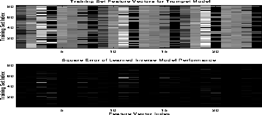
Figure 4 shows an image-map of the
original training set of sound feature vectors, and the square-errors
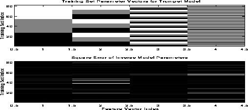
of the output of the system after training. Figure 5
shows the relationship between the parameter vectors of the training set and
the estimated parameters of the inverse model.

Figure 4: Image map of the outcome errors of the inverse estimator after training.
The upper image shows the feature vectors from the training data and the lower image
shows the square error of the outcome of the distal learning system with respect
to the original feature vectors. Brighter areas indicate higher error.

Figure 5: Image map of the parameter errors of the inverse estimator after training.
The upper image shows the parameter vectors from the training data and the lower
image shows the square error of the estimated parameters with respect to the
original parameter vectors. Brighter areas indicate higher error.
The mean-squared error of the parameter estimates was  with a
variance of
  . Table 2 shows an
analysis of the variance of each parameter. The mean-squared error in
the sound signal after resynthesis from the estimated parameters was
 , and the variance was
  . The relatively high variance
of the sound errors after resynthesis from parameters with low mean
and variance is accounted for by variances in the sound
representation. The auto-regressive model estimator that was used for
extracting the parametric representation for sound had a high variance
with respect to a steady input source, and the physical model itself
had a high variance with respect to steady input parameters.

Table 2: Analysis of Parameter Errors for the Brass Model
In order to test the generalization ability of the inverse modeling
system, an additional 81 test waveforms were generated using the Korg
Prophecy synthesizer and these were fed to the function
approximator. The results showed that the inverse estimator functional
approximation was able to interpolate successfully in order to obtain
accurate parameters for novel sounds that belong to this class.


Next: Discussion
Up: Experiment 1: Single Model
Previous: Method
Michael Casey
Fri Mar 22 15:49:22 EST 1996


