DNA Sequencing Quality Control Analysis

I used an exercise working with sample quality control data concerning DNA sequencing runs from a genomics company as an opportunity to practice data handling in Pandas. The raw data consisted of three hundred .txt files each corresponding to a 96-well plate's worth of sequencing reactions. Each sequencing reaction was labeled with a unique identifying bar code, an indication whether the sample was collected from blood or saliva, the size in DNA base pairs of the fragment sequenced, the pre- and post- library amplification DNA sample concentrations, and several additional QC flags, including "coverage" and "CNV calling".

First, I extracted all the data and read it into a data frame for all further handling. I determined that 93.76% of the reads had passed both quality control flags, 1.25% had failed at the coverage flag, and the remaining 5.00% had passed coverage but failed the CNV calling flag.

Running a χ² test for independence on each of the two tables results in p-values of 5.4×10^-31 and 0.52 respectively, indicating that passing the coverage flag is dependent on sample type (failure being more likely for saliva samples than for blood) but that the sample type has no evident effect on passing CNV calling.

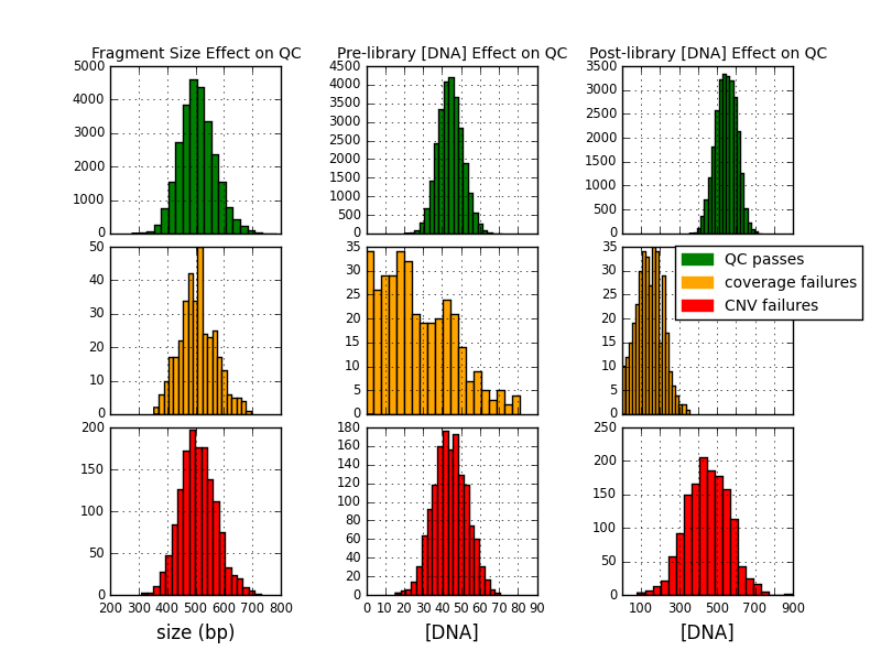
Next, I grouped the data into the set that passed both QC flags, the set that failed the sequencing coverage flag, and the set that passed sequencing coverage but failed CNV calling. Then, for each of the three metrics—fragment size, and pre- and post-library amplifcation concentration—I plotted the histogram in terms of that metric for each of the three states corresponding to the different failure/passing combinations, and aligned the three distributions in a column. The three pass/fail states have similar distributions in terms of fragment size, so that doesn’t appear to be a factor. The set that only failed CNV calling has a similar pre-amplification DNA concentration distribution to the set that passed both QC flags. However, in the set that failed the coverage flag, the pre-amplification average concentration is significantly shifted to the left (the variance is also clearly greater and overall this histogram deviates much more obviously from a normal distribution than the other eight). This shift (though not the deviation from normality) is even more apparent in the post-amplification DNA concentration column, where the distributions in the coverage failure set and the passing set are essentially distinct with negligible overlap. The distribution of the set that failed CNV calling has much more overlap with the set that passsed both flags than the group that failed coverage, but it’s still significantly shifted to the left, so that the majority of its population occupies the space between the other two distributions.

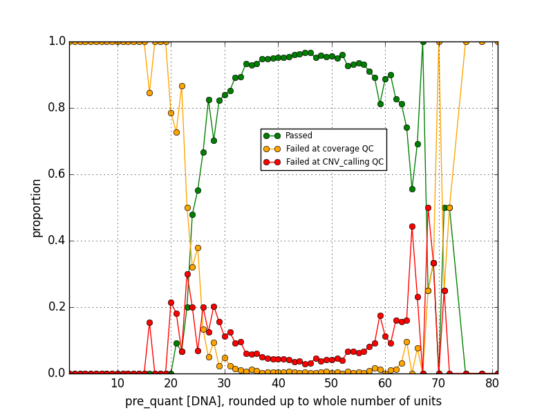
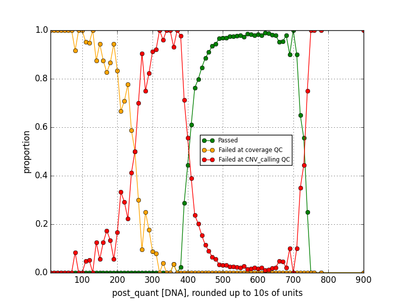
Then I looked at the data in the pre- and post- DNA concentration sets a different way by allocating them into bins with a width of 1 (for pre-amplification) or 10 (for post-amplification) concentration units, and calculating the proportion of data in each bin corresponding to each of the three pass/fail states. From there I can estimate the probabilty of a future sequencing reaction with a given DNA concentration passing, or failing with either of the two QC flags. I can summarize some rough rules of thumb: a pre-amplification DNA concentration less than about 22 or 23, or a post-amplification concentration less than about 230 or 240, means the sample will most likely fail with a coverage flag, while a post-prep concentration higher than 240 but less than around 400 is most likely to fail with a CNV calling flag. Reactions with intermediate concentration ranges pass with 90-95% success rates, and then at the higher concentration ranges—greater than 67 pre-amplification or greater than about 740 or 750 post-amplification— failures become more common than not again. This sort of data analysis could be used to improve efficiency by removing reactions that are unlikely to work from the pipeline before resources are wasted on them.

In terms of programming techniques, this exercise gave me extensive practice working with dataframes, and provided me the opportunity to practice the statistical analysis and graphing methods associated with them.