Undergrad math, and the variance lens of deep learning

Someone asked me how high school or undergrad math shows up in deep learning.

The calculus chain rule underpinning backprop is the classic example. Matrix decomposition to explain exploding or vanishing gradients is another good one. RoPE embeddings for transformers were introduced recently, which use complex numbers in their formulation, plus an application of rotation matrices.

Having a grasp on the fundamentals allows you to both (1) understand the mechanics and behavior of neural networks, but also (2) work on the edge of research.

Another example: the variance lens of deep learning

A lot of tricks in deep learning are really the same idea wearing different costumes. Here's one where the idea is simple: keep the variance of the signal roughly constant as it flows through the network.

Every time a network sums up many things — a dot product, a residual stream, a gradient over a batch — the scale of the result drifts by \(\sqrt{n}\) unless you do something about it. The "something" is what gets a name. These corrections are needed due to the simple fact that if you add \(n\) independent, zero-mean random variables each with variance \(\sigma^2\), the variance of the sum grows linearly.

Costume 1 — Attention's 1/√d, LayerNorm, and other normalization methods

We can spell this out for Attention's 1/√d term by using variance identities one might learn in an introductory class:

• Sum identity: \( \operatorname{Var}(A+B) = \operatorname{Var}(A) + \operatorname{Var}(B) + 2 \operatorname{Cov}(A,B) \).
• Product identity: \( \operatorname{Var}(A * B) = \operatorname{Var}(A) * \operatorname{Var}(B) + \operatorname{Var}(A) * E[B]^2 + \operatorname{Var}(B) * E[A]^2 \).
• Constant multiplier identity: \( \operatorname{Var}(c*X) = c^2 * \operatorname{Var}(X) \)

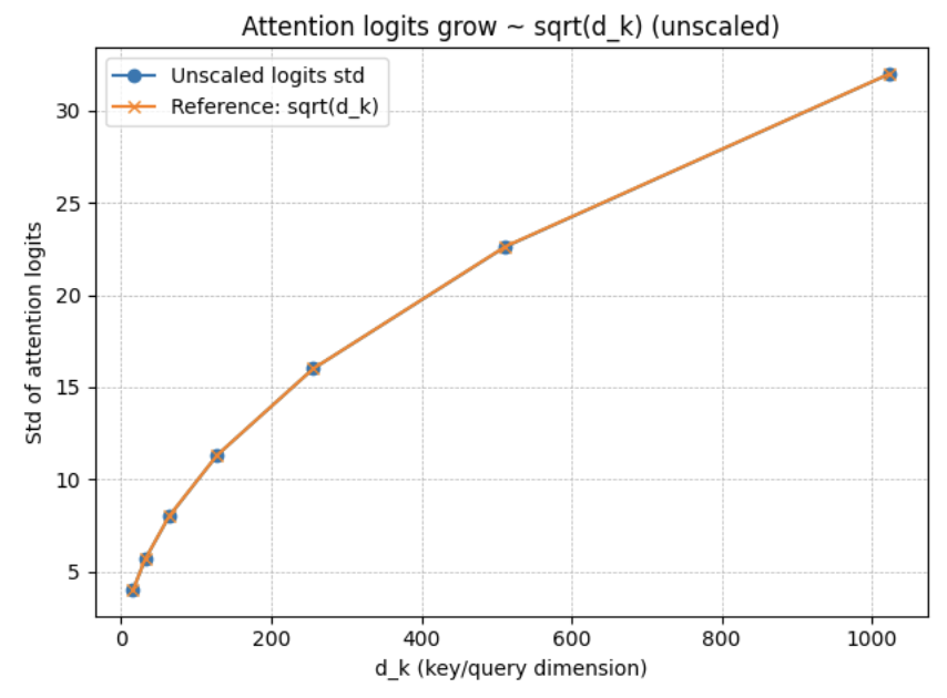
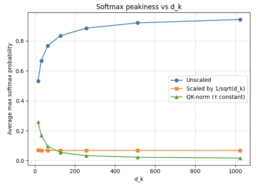
Scaled dot-product attention computes scores \(q \cdot k = \sum_{i=1}^{d} q_i k_i\). Assuming the random vectors are independent and have unit variance, we can use the sum and product identities to state \( \operatorname{Var}(A_0*B_0 + \dots + A_d*B_d) = \sum \operatorname{Var}(A_i * B_i) = d \). Using the constant multiplier identity, we arrive at dividing by √d (and not d) in order to main unit variance.

The bad effects of (not) keeping the variance constant are shown below:

Costume 2 — Initialization

The same logic applies for initialization. A linear layer computes \(y_j = \sum_{i=1}^{d_\text{fan\_in}} W_{ji}\,x_i\). To keep the output at unit variance, we need \( \sigma_W^2 = \frac{1}{d_\text{fan\_in}} \).

That is exactly Lecun initialization. He init makes the same argument, but with a scaling factor of 2 to account for ReLU killing half the signal. This only accounts for forward pass variance, so Xavier/Glorot init average over fan_in and fan_out to manage backward pass variance as well.

(Bonus) Costume 3 — Batch size and learning rate

A minibatch gradient is an average of \(B\) per-example gradients. Averaging \(B\) independent, variance-\(\sigma_g^2\) estimates gives a gradient whose variance is \(\sigma_g^2 / B\) — i.e. its noise scale falls like \(1/\sqrt{B}\). To keep the size of each noisy update roughly fixed when you grow the batch, you scale the learning rate like \( \eta \;\propto\; \sqrt{B}. \).

Note that I've listed this as a "Bonus" costume. Alternatively, the widely used linear rule ($\eta \propto B$) focuses on expected value rather than variance, allowing a single large-batch step to travel the same distance as several small steps in highly noisy regimes. Both rules eventually break down once the batch size exceeds the Gradient Noise Scale, at which point the variance becomes negligible and the learning rate is strictly capped by the curvature of the loss landscape.