What Was I Thinking?, a memory-prosthesis project at the MIT Media Lab, is studying what triggers a person’s memory of something said in a conversation. Some memory triggering functions that are being tested include the occurrence of laughter, the people present during the conversation, or activity during a conversation. Recalling that laughter took place during a conversation could remind the person that something funny was said. Recalling that a number of people were present during the conversation could remind the person of something important that was said during a meeting.
Another potentially useful memory trigger could be knowing the location of the conversation or whether movement took place during the conversation. For example, if a person remembers that a conversation took place in their office instead of at the water cooler, this information could possibly remind them of something in particular that they are trying to recall.
Location sensing using a wireless network has many applications beyond use in memory prosthesis. For example, visitors could download a building map upon entering a building for the first time and then track their progression through the building. Location sensing could also be used for nearest-resource location, (e.g. finding the nearest printer for your mobile laptop). Additionally, system administrators could locate wireless devices when necessary. For example, last summer, the MIT Media Lab was hit by the Code Red virus. There was a portable computer in the lab connected to the network via the 802.11b wireless network that was continuously sending out copies of the virus, but the system administrators were unable to locate the computer for some length of time because the computer was not set to a know location.
What Was I Thinking? uses an iPaq™, a palm-sized computer, to record and save an audio conversation, the time and location of its occurrence, and user-defined markers in the conversation. To determine the location of the iPaq, the existing 802.11b wireless computer network in the MIT Media Lab is used. The 802.11b wireless network consists of a number of access points (or base stations) scattered about a building. Access points are placed in known, fixed locations where they are connected to the wired network (see Figure 1).
Figure 1 Configuration of access points connected to a wired network. Wireless devices communicate with the wired network through the access points. [1]
From any point covered by wireless access, a wireless device can hear one or more access points with varying signal strengths. The closer the wireless device is to an access point, generally the stronger the signal received from that access point is. Previously, to determine the location of the iPaq, it was assumed that the access point from which the iPaq was receiving the strongest signal was the one the iPaq was closest to. Therefore the iPaq was in the room that contained that access point. The precision of this method depends on the number and location of access points in relation to the room configuration. Rooms and labs that do not have their own access points are indistinguishable from the closest room or lab with an access point. If room B and room C’s closest access point is in room A, then the iPaq will report that it is in room A if it is in room A, B or C (Figure 2).
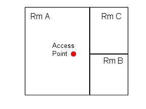
Figure 2 Simple configuration of three rooms and one access point. While rooms B and C may be covered by wireless access, it is impossible to tell the difference between rooms A, B, and C using a single access-point method.
II.A Non 802.11b
Previous work using signal-based location sensing includes using infrared (IR) sensors, cell phones, and Global Positioning Systems (GPS). As most of the signal-based location sensing technology was developed with the intention being used for navigation, most current techniques require extra hardware that is not commonplace or cannot be used indoors. For example, IR networks such as "Active Badge"[2] or combination of IR and 802.11b networks such as SpotON [3] require that the whole room or building be outfitted with IR sensors, which adds additional overhead. While IR sensors have high precision, IR sensors do not have a very wide range; therefore, many sensors are needed around a room or building. GPS requires that the receiver has line of site access to orbiting satellites [2, 4] and is therefore limited to outdoors. The walls of buildings and even tree canopies can block GPS signals. Recently there has also been work done to locate cell-phone users and determine their position should they make a 911 call. However cell-phone location technology is still being developed. Cell phones also do not work in every building due to cell signals being blocked by the building walls.
The advantage of location sensing using the wireless 802.11b network is that many office buildings are already equipped with wireless access. Therefore, a software-only solution may be deployed to create a signal-based location-sensing system within a building.
II.B 802.11b
Previous location-sensing systems using the wireless 802.11b network includes the RADAR project at Microsoft, the Nibble project at UCLA, and Advanced WaveLan Positioning, a student project at Luleå University of Technology. The Microsoft RADAR project created a radio-frequency (RF) map of signal strength data at 70 locations on a floor [5]. To handle mobile users, the RADAR project kept track of the user at all times, comparing results from current signals to results of the previous five signals. This history-based method was an effective solution to signal aliasing (two or more locations having the same signal strengths from available access. To determine where users were based on current signal strengths, RADAR used k-nearest neighbors with an added weighting factor based on the inverse of the distance of the newest point from the last known point. RADAR’s accuracy was within 5 m (16.4 ft) 75% of the time [6].
The Nibble project also created and used an RF map of signal-strength data around their lab. Nibble then used a Bayesian network to determine where the user was. Their stated accuracy was within 3 m (10 ft) [7].
The Advanced WaveLan Positioning student project at Luleå University of Technology tried using both an RF map and triangulation based on RADAR’s research on wall attenuation factors (WAF). Triangulation yielded an accuracy of 8 m (26 ft) [8].
All projects limited their domain to a single story of a building. The RADAR project did briefly test a three-story environment where all access points within each floor were placed in the same place on each floor. RADAR found that because the floors were so thick, most of the signals from surrounding floors were blocked.
I build on these results by expanding the domain to multiple stories of a building, analyzing the differences between classification methods, and experimenting with using a signal-based location-sensing system in the real world, as opposed to just confining it to a laboratory conditions.
III.A Theoretical – Accuracy
When a wireless card is queried about nearby access points, it returns all access points in range and the strength of the signal that it receives from these access points. Access points in range are determined by signals in response to a packet sent out from the wireless card. Signal strength is calculated through a combination of signal levels and signal-to-noise ratio calculations.
A wireless card and an access point each have signal outputs of 15 dBm and receiver sensitivity of –82 dBm. [9] In the United States, the legal limit on the strength of the signal output of any wireless device in the 2.4 GHz range limits the range of the signal to approximately 500 feet.
The signal strength of a radio wave degrades over distance in space. This degradation can be modeled by the free-space path-loss equation that provides signal attenuation through free space or a vacuum (Equation 1).
FSL = [36.6 +20log(f) + 20log(d)]
Equation 1 Where f is the frequency of the radio wave in MHz, and d is the distance in miles. [10]
Given that we are working with signals in the 2.4 GHz range, the free-space loss of our access points to wireless cards can be modeled as shown in Graph 1.
Graph 1 Signal Degradation in Free Space
Given this model, we can theoretically determine how far our wireless card is from an access point by the signal strength loss over space. However, since the signal-strength number returned by most wireless cards is an integer, we lose accuracy the farther we are from access points. For example, if we are within 13 feet of at least three access points, we can calculate our position with and error of plus or minus one foot. We can remain accurate up to three feet if we are within 46 feet of at least three access points. At approximately 300 feet, calculations based on signal-strength degradation become less accurate than GPS. (See Table 1).
Using the data from Table 1 we can now predict where we are within a building and know how accurate our calculation is given signal strength information from at least three access points. When equidistant from three or more access points, we can predict that we are within a somewhat circular area of a known radius. When not equidistant from three or more access points, we can predict that we are within an oblong area depending on which access points we are closest to.
Table 1 Theoretical accuracy of measuring distance from access points based upon signal strength
|
Accuracy (ft) |
|
|
13 |
1 |
|
23 |
2 |
|
46 |
3 |
|
65 |
4 |
|
73 |
5 |
|
300 |
16.4 |
|
400 |
23 |
|
5280 |
287 |
We can determine the theoretical limits of location sensing within a building by determining where we are within a range of at least three access points. Given the network topology of the MIT Media Lab (see Section IV.A) it was predicted that the best accuracy should be areas in the central portions of the third and fourth floors such as the Garden, the Pond, and the lab in 446. Areas with the worst accuracy should be areas on the lower level such as the Holography Lab and the lobby.
III.B Theory vs. Practice
The theoretical accuracy of signal-based location sensing does not map well to practice. In reality, simple triangulation based on free-space signal loss does not work in the Media Lab. None of the aforementioned calculations took into account any wall or floor attenuation factors, mobile objects such as people, or any other objects in the building that absorb or reflect radio signals.
When a radio signal hits an object straight on, the signal can be absorbed, reflected, or some combination of the two. If a radio signal hits an object at an edge, the signal may be diffracted. When there are many objects in the signal path, the signal may be scattered (see Figure 3-5).
Figure 3 When a signal passes through an obstruction, some of the signal is reflected back, and some of the signal passes through the obstruction [11].
Figure 4 If a signal hits an obstruction at an angle, the signal may be diffracted and continue at a different angle [11].
Figure 5 If a signal hits numerous objects in an enclosed space, the signal may be scattered in many different directions [11].
Different materials can cause different levels of attenuation to a radio signal. Examples of such attenuation are shown in Table 2.
Table 2 2.4 GHz Signal Attenuation through various obstructions [2, 11]
|
Office Wall |
6 dB |
|
Metal Door in Office Wall |
6 dB |
|
Cinder Block Wall |
4 dB |
|
Window in a Brick Wall |
2 dB |
|
Human |
4 dB |
Given signal attenuation factors of various objects, it is possible to build a better theoretical map of a building based on the layout of the building; however, this is difficult to do in practice.
IV.A Setting – MIT Media Lab
The Wiesner building, which houses the MIT Media Lab, is approximately 100 ft high, it has five levels each approximately 20 ft high. There are approximately fifteen large open labs, over 100 smaller offices, a large atrium, as well as two stairwells and 3 elevators. Office doors are either metal or glass. Most office walls are sheetrock, some are constructed from glass.
The population density of the MIT Media Lab varies greatly during a week. Most weekdays during business hours there are a number of visitors in the Media Lab. During weekends and non-business hours, the lab is mainly populated by students and faculty.
There are 15 access points distributed around the building. Four on the lower level, none on the first floor (which contains the List Visual Arts Gallery), one on the second floor, six on the third floor, and four on the fourth floor. The access points are not evenly distributed over each floor; as wall and floor signal attenuation, and bleed (many of the floors and walls in the Media Lab are not very thick) cause some access points to have a very limited range and others to be usable as the primary base station by a user a floor away. In fact some access points were purposely placed so as to cover the floor above or below its location, as well as its immediate surrounding area.
IV.B Experimental Subjects
One subject was used in testing the location-sensing software. The device was handed to a sponsor during a Media Lab demo day. The sponsor only traveled to major lab areas and moved from lab area to lab area through the main hallways. The sponsor did not spend much time in the hallways during transit. Once in a lab area, the sponsor would stay in about the same spot for a number of minutes (5–10) before moving on to a different spot within the Media Lab.
IV.C iPaq
The device that was used for this project was an iPaq running Familiar 0.5 (a version of Linux for iPaqs) with a Cisco Aironet 350-series wireless card. The Familiar operating system was chosen because it allowed multiple access points to be accessed simultaneously. To obtain signal strength information, we used the wireless tools written by Jean Tourrilhes at HP [12]. From most points in the lab, we can receive signal-strength information from one to a maximum of eight access points around the lab.
IV.D Laboratory
The Laboratory phase had two parts: offline data collection and calibration and online usage.
IV.D.1 Calibration
In the offline phase the iPaq was used to collect signal-strength data at known points around the lab. Initial calibration tests were run in the Garden (one of the main lab areas of the Media Lab, it measures approximately 30 feet by 40 feet) to determine which density of calibration points had the best accuracy levels. Three levels of calibration were tested, one point every ten feet, one point every 20 feet, and one point every 30 feet. Each point was calibrated with twenty pieces of data, five in each of the cardinal directions (as the RADAR paper had showed that orientation did have an effect on signal strength received [5]). A calibration point at every 20 feet was determined to have the best accuracy (Table 3).
Table 3 comparison of classification method used, granularity of calibration and average percentage correctly classified within 10 feet of actual location.
|
10 feet |
20 feet |
30 feet |
|
|
1-Nearest Neighbor |
64% |
60% |
63% |
|
3-Nearest Neighbors |
70% |
71% |
65% |
|
5-Nearest Neighbors |
68% |
71% |
60% |
|
Naïve Bayes |
70% |
72% |
62% |
|
Neural Network |
72% |
63% |
N/A |
These results were significant to p = 0.004. Based upon these results, a larger portion of the lab was calibrated over three floors (a small part of the 2nd, and half of the 3rd and 4th floors) that overlay each other. After testing the accuracy of the larger portion of the lab, most of the Media Lab was calibrated over 5 floors. Areas that were left out were areas that most people did not have access to.
IV.D.2 Classification
The calibration data was sent to a database on a separate computer. Once the data was in the database, a classification system was created. To figure out which classification system was to be used, a few classification methods were tested by using WEKA, a data mining toolkit. Five types of classification were tested: 1-Nearest Neighbor, 3-Nearest Neighbors, 5-Nearest Neighbors, Naïve Bayes, and Neural Networks. The results of these tests are listed below in Table 4.
Table 4 Comparison of classification methods and average percentage correctly classified within 10 feet of actual location.
|
1-Nearest Neighbor |
62.1% |
|
3-Nearest Neighbors |
68.8% |
|
5-Nearest Neighbors |
66.3% |
|
Naïve Bayes |
68.1% |
|
Neural Network |
67.6% |
Overall, 3-Nearest Neighbors appeared to have the best results. These results were not statistically significant (p = 0.08). However, we decided to use Naïve Bayes because it allowed us to use prior probabilities, an important feature if we are to use user profiling.
IV.D.3 Testing
To test the accuracy of our system on a small scale, test data was taken at ten-foot intervals at random orientations over 3 floors that had previously been calibrated. Using the WEKA toolkit the data was classified using four of the five classification methods previously tested (Nearest Neighbors, 3-Nearest Neighbors, 5-Nearest Neighbors, and Naïve Bayes). The classified data was then compared with the known location of the test point. If a point was classified within 10 feet of its actual location, it was considered correct.
IV.E Real World
To see how well signal-based location sensing worked for a person traveling through the Media Lab, the iPaq was handed to a sponsor during a demo day at the Media Lab. The iPaq was set to continuously record the signal strengths of the access points it could hear and send them to a server every 15 seconds. The sponsor was also shadowed to record the actual location of the sponsor. In this manner we were able to test the accuracy or our system by using classification methods to determine their location given the signal strength data, and then compare it to the actual location of the user.
IV.E.1 User Profiling
People are somewhat predictable in their locations throughout the day. For example, a person whose office is located on the third floor is much more likely to be found at the third floor coffee room than the second or first floor coffee room. People also spend more time in offices than in hallways. Within the Media Lab, a student or professor whose office is in one corner of the lab is more likely to be found in that corner of the lab than a section that is located at the other end of the building. This knowledge can be taken into effect in a location system by using a user’s habits to predict more accurately where a user is more likely to be.
There is also a simpler, temporal prior probability. A user who is determined to be in a particular location is fairly unlikely to be more than 20 feet or a floor from that location in the next 10 seconds. The RADAR project at Microsoft takes this knowledge into account in their history-based tracking. RADAR uses the Euclidean distance between two points as the weighting factor of the likelihood of the transition. The greater the weight, the less likely the transition [6].
To implement user profiling in our system, it was planned that the data from the sponsor shadowing would be used to create a profile for the sponsor. The percentage of the total amount of time spent at any location would be that location’s prior probability. For most smaller spaces, a users’ profile would indicate a uniform likelihood of being at any one point in the space. For larger spaces, a user profile may show a person to be more likely to be in one corner than the other. Bayesian classification methods can be used to classify the user’s location based upon the current signal strengths and the prior probabilities of that location.
The WEKA toolkit explorer doesn’t support prior probabilities however, so user profiling has not yet been put into practice.
V.A Laboratory Results
V.A.1 Accuracy overall
Two hundred eighty-nine points in the Media Lab were tested. Laboratory accuracy was determined by comparing classified data with the known test location. If a point was classified within 10 or 20 feet of its actual location, it was considered correct. A breakdown of accuracy is in Table 5 below.
Table 5 Comparison of classification methods and average percentage correctly classified within 10 and 20 feet of actual location
|
Within 10 ft |
Within 20 ft |
|||
|
# Correct of 289 |
% Correct |
# Correct of 289 |
% Correct |
|
|
Nearest Neighbors |
195 |
67.4% |
242 |
83.7% |
|
3-Nearest Neighbors |
186 |
64.3% |
237 |
82.0% |
|
5-Nearest Neighbors |
180 |
62.3% |
239 |
82.7% |
|
Naïve Bayes |
181 |
62.6% |
241 |
83.3% |
While 1-Nearest Neighbor had the best overall results, these differences were not statistically significant (p = 0.06).
After the small-scale test, a larger scale test of the entire Media Lab was performed. One thousand, six hundred twenty-three points were tested. Points were classified using only Naïve Bayes as it had previously been determined that the classification method had little significance on overall accuracy (See Table 6).
Table 6 Accuracy Lab wide using Naïve Bayes classification
|
Within 10 ft |
Within 20 ft |
|||
|
# Correct of 1623 |
% Correct |
# Correct of 1623 |
% Correct |
|
|
Naïve Bayes |
1182 |
72.83% |
1409 |
86.81% |
Some areas of the lab were more accurate than others. Hallways were the most accurate places. Most points in hallways were accurate within 10 feet. Larger lab areas were generally more accurate than smaller offices. The edges of the larger rooms (near walls) were generally more accurate than the middle of a room. There were also noted differences in accuracy by location by classification method. Naïve Bayes generally did better than any of the Nearest Neighbors methods in areas with sparse data (few access points available from that location) while the Nearest Neighbors methods did better than Naïve Bayes in areas with strong connectivity (many access points available from that location).
V.B Real World Results
V.B.1 Accuracy overall
Four hundred sixty-seven data test points were collected during the sponsor shadow experiment. The data was classified using Nearest Neighbors, 3-Nearest Neighbors, 5-Nearest Neighbors, and Naïve Bayes. Accuracy was determined by comparing classified data with the known test location. A breakdown of accuracy and classification method used is shown in Table 7.
Table 7 Comparison of classification methods and average percentage correctly classified within 10 and 20 feet of actual location
|
Within 10 ft |
Within 20 ft |
|||
|
# Correct of 467 |
% Correct |
# Correct of 467 |
% Correct |
|
|
Nearest Neighbors |
182 |
38.97% |
250 |
53.53% |
|
3-Nearest Neighbors |
180 |
38.54% |
242 |
51.82% |
|
5-Nearest Neighbors |
161 |
34.48% |
240 |
51.39% |
|
Naïve Bayes |
169 |
36.19% |
290 |
62.10% |
These results are significantly worse than laboratory results. There are a number of reasons for this discrepancy. The lab was calibrated when there were fewer people in the lab compared to a demo day where the number of people in the lab may more than double. Previous work has shown that the number of people in an area can affect the accuracy of a signal-based location system as people do cause signal attenuation [6]. The sponsor also spent most of their time in the major lab areas, which are not as accurate as other portions of the lab such as hallways (V.A.2 Accuracy by location).