Grocery shopping and the resupply model

Online grocers and other retailers whose products are delivered have a very different cost structure than traditional brick-and-mortar stores (Boatwright et al, 2002), requiring them to develop new policies for pricing and promotion. Fortunately, delivery retailers tend to have detailed information about their customers' buying habits, because each purchase is tied to an address. Hence there is an opportunity to use data mining to set price/promotion policies.

A first step toward this goal is to develop a model of an individual's purchasing behavior. As described by Boatwright et al, delivery retailers need models not just of total sales but of the relationship between purchase quantity and purchase frequency. This is because a delivery retailer can increase profits not just by increasing total sales but also by reducing purchase frequency.

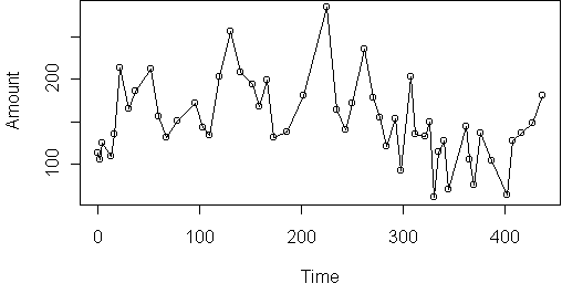
The dataset used here is the same one used by Boatwright et al. It describes the purchase dates and amounts for 14,000 different customers of an online grocer during the years 1996-1998. Here is the data for one of the customers (aa16755):

Time Amount
   0 112.98
   3 105.37
   5 125.07
  14 109.84
  17 135.89
...

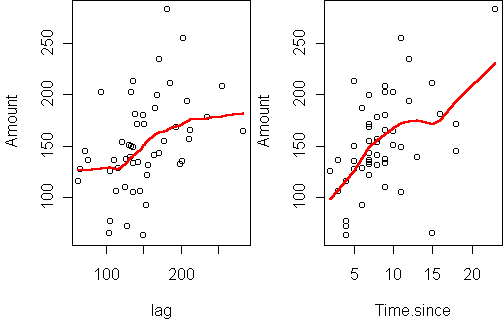
Time is in days and has been standardized so that the first purchase date is 0. Amount is in dollars. The only thing you can really see in this plot is that the amounts are generally high in the beginning and low at the end.

A better approach is to plot the amount versus the lagged amount and versus the time since the last purchase:

This shows a strong connection with time and a lesser positive correlation with the previous amount. A linear autoregressive model, which predicts Amount based on the previous purchase amount and the time since, can explain 36% of the variance.

However, an autoregressive model is not an intuitively appealing model of purchasing. So we turn to a different model, in hopes of better performance.

Resupply model

Intuitively, the purchase amounts should be related to the customer's needs at the time. In other words, they should be related to the customer's supply. Of course, the store never observes the customer's supply, but by making some assumptions about the customer, it is possible to infer their supply. Consider the basic supply equation:

Supply = Initial.supply + Total.purchases - Consumption

The first assumption is that the customer has a constant consumption rate:

Consumption = Rate * Time

The second assumption is that the customer makes purchases in order to minimize the variance of their supply. In other words, the customer minimizes the sum of squares of the supply over time. The third assumption is that the customer is loyal, i.e. they always purchase these particular products at this particular store. Hence the store knows the customer's total purchases. Because we know the total purchases and we know the time, we can rewrite the supply equation into a linear regression problem:

Total.purchases = Rate * Time - Initial.supply + Supply

where Rate is the slope, -Initial.supply is the intercept, and Supply is the "noise" (the residual of the fit).

To check that these assumptions are valid, it is sufficient to plot the customer's total purchases over time, and see if it is linear:

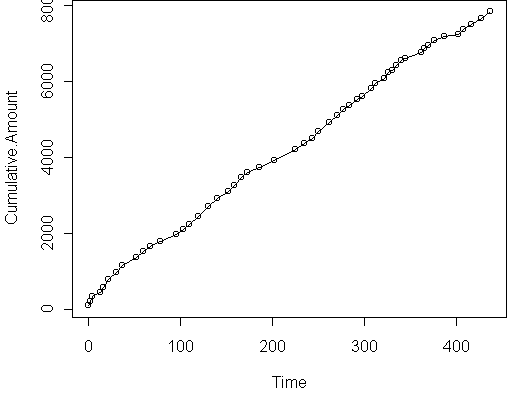
This curve is not perfectly linear, but it does follow locally linear trends.

Estimating supply

To get a more detailed picture, it helps to look at the residuals of the model (which is the supply immediately after each purchase):

Supply is only recoverable up to an additive constant, so don't take the supply values literally. This plot is based on a consumption rate of 21, chosen to give residuals which are locally flat. There are intervals in which the supply is roughly constant. In between these intervals, the supply suddenly changes, suggesting a change in consumption rate, or equivalently a change in loyalty. Most likely, the customer shopped elsewhere during these periods.

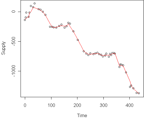
An interesting by-product of the resupply model is that we can estimate exactly when the customer shopped elsewhere and how much they spent. To do this, we add extra terms to the regression model representing a sudden change in supply at a particular time. Stepwise regression can automatically tell us which terms are useful. Doing this for the above customer produces the model

(Intercept)         Time     Time.402     Time.362  
     251.72        20.57      -382.36      -213.14  
    Time.96     Time.225     Time.202  
    -246.77      -237.19      -229.81

The coefficient for Time is the consumption rate. The Time.X terms are step functions which begin at a particular time. This implies disloyalties at times 96, 202, 225, 362, and 402, with values $247, $230, $237, $213, and $382.

The learned model leads to the following estimate of supply over all time (disloyal periods omitted):

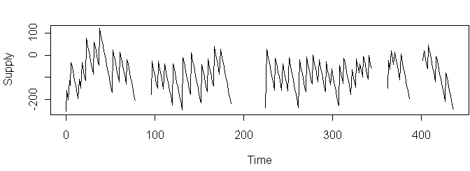
The assumption of constant consumption rate is evident in the zigzag shape.

Predicting purchase times

Using this new supply variable, we can try to predict when the customer will make a purchase. (For this to be valid, the supply on a purchase date must be the pre-purchase supply.) The approach taken here is simply a logistic regression which predicts, per day, whether a purchase will be made that day. The predictors are supply and time since the last purchase. Here is the result:

             Estimate Std. Error z value Pr(>|z|)    
(Intercept) -4.471736   0.469943  -9.515  < 2e-16 ***
Supply      -0.011797   0.003809  -3.097  0.00195 ** 
Time.since   0.220338   0.067869   3.247  0.00117 **

The probability of purchase depends on both time and supply, in the expected directions: a purchase is more likely when the time since is long and the supply is low.

Predicting purchase amounts

Here are scatterplots of the purchase amount versus pre-purchase supply and the previous purchase amount:

To predict the amount, we use a linear regression, with the same two predictors:

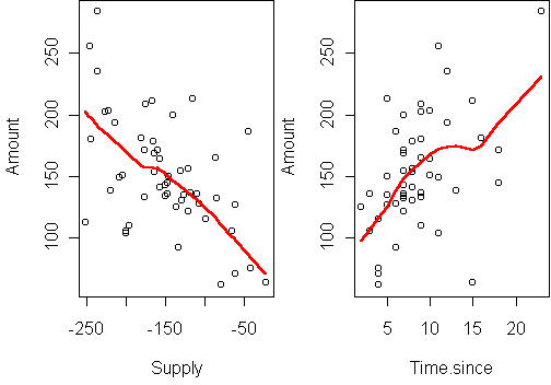
            Estimate Std. Error t value Pr(>|t|)    
(Intercept)  68.1482    15.0875   4.517 4.09e-05 ***
Supply       -0.3915     0.1021  -3.835 0.000365 ***
Time.since    2.9479     1.3462   2.190 0.033428 *

Again the directions are intuitive. Note that supply is the most significant predictor. The R-squared of this fit is 42%.

So not only does the model give information about loyalty, it also gives a better fit than autoregression. The actual predictive performance, however, is unknown since the supply was estimated from the entire dataset, not just the data prior to each amount. A full treatment of this latent-variable model would estimate supply sequentially, and perhaps allow the consumption rate to change over time.

Other customers

This analysis involved only one out of 14,000 customers in the dataset. Other customers show various different behavior. For example, some have purchase frequencies which depend on supply but the amounts do not. Others have purchase amounts which depend on supply but the frequency does not. Some have a very non-constant consumption rate and cannot be handled at all.

A next step would be to automate fitting the resupply model and recover coefficients for each customer, describing the extent to which their purchases depend on supply versus time, and their loyalty. This would give a map of the typical purchasing behavior for the customers of this online grocer.

References

Peter Boatwright, Sharad Borle and Joseph B. Kadane, "A Model of the Joint Distribution of Purchase Quantity and Timing", CMU Department of Statistics Technical Report #741, 2002.

Tom Minka

Last modified: Tue Dec 03 16:12:27 EST 2002