In particular, we will look for outliers. For univariate data, outliers are easy to spot by sorting the residuals. For multivariate data, the residuals are also multivariate, so how do we define "most unusual"? One idea is to use the multivariate length of the residual: ||x - xhat||. This doesn't quite work because it doesn't consider that different variables might have different amounts of spread, and that they might be correlated.
The multivariate normal distribution can be used to define outliers, just as with the univariate normal. In both cases, an outlier is a value whose probability is unexpectedly small. In the univariate case, this is a point far from the mean, in either direction. In the multivariate case, this is a point far from the mean, where some directions count more than others. Directions with large spread require the point to be farther away before it is considered an outlier.
The procedure is thus: fit a multivariate normal distribution to the dataset, compute the probability of each point, and flag the points whose probability is unexpectedly low (using p-values). The function outliers does this.
> x[1,]
              Price MPG.highway EngineSize Horsepower Passengers
Acura Integra  15.9          31        1.8        140          5
              Length Wheelbase Width Turn.circle Weight
Acura Integra    177       102    68          37   2705

> i <- outliers(x)
                         D2      p.value
Chevrolet Corvette 38.21730 3.478412e-05
Mercedes-Benz 300E 34.44389 1.552920e-04
Dodge Stealth      33.78617 2.007485e-04
Mazda RX-7         32.53516 3.259493e-04
Ford Aerostar      30.49141 7.115836e-04
Geo Metro          23.73304 8.341393e-03
Chevrolet Astro    21.18824 1.981855e-02
Mercury Cougar     19.54928 3.381575e-02
Honda Civic        19.36320 3.588471e-02
Volkswagen Eurovan 18.64282 4.504106e-02
These cars all have p-values less than 5%, meaning that their probabilities
are so low that we would expect a multivariate normal dataset of this size
to have such cars less than 5% of the time.
For each outlier car, we would like to know what makes it different from the rest of the data: is it an unusual size, unusual price, etc.? In general, if you want to know what makes two groups different, you can think of the groups as classes and use classification methods to distinguish them. Let's use discriminative projection:
i <- outliers(x)[1]
x$cluster <- rep(F,nrow(x))
x[i,"cluster"] <- T
x$cluster <- factor.logical(x$cluster)
sx <- scale(x)
w <- projection(sx,2,type="m")
cplot(project(sx,w),axes=F)
plot.axes(w)
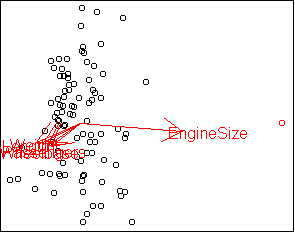
We can avoid typing the above sequence of commands by using the convenience function separate. Let's look at the second outlier car:
> i <- outliers(x)[2]
> separate(x,i)
      Price       Width  Passengers MPG.highway   Wheelbase
-0.84792449 -0.24664714 -0.12396093 -0.05775463 -0.02421979
Turn.circle  EngineSize      Length      Weight  Horsepower
 0.06843721  0.07269870  0.16373487  0.27272652  0.29957158
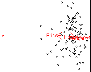
Finally, the third outlier car:
> i <- outliers(x)[3]
> separate(x,i)
   Wheelbase   EngineSize        Price  Turn.circle        Width
-0.489502780 -0.275354612 -0.195988691 -0.026335603  0.002412840
      Length   Passengers  MPG.highway   Horsepower       Weight
 0.015204207  0.124316064  0.194260598  0.418239977  0.645839301
The Dodge Stealth is unusual because it has the Price, EngineSize, and
Wheelbase of a coupe but the Horsepower and Weight of a sports car.
sx <- scale(x)
hc <- hclust(dist(sx)^2,method="ward")
cluster <- factor(cutree(hc,k=4))
y <- x[cluster==1,]
> y
               Income Illiteracy Life.Exp Homocide HS.Grad Frost
Alabama          3624        2.1    69.05     15.1    41.3    20
Arkansas         3378        1.9    70.66     10.1    39.9    65
Georgia          4091        2.0    68.54     13.9    40.6    60
Kentucky         3712        1.6    70.10     10.6    38.5    95
Louisiana        3545        2.8    68.76     13.2    42.2    12
Mississippi      3098        2.4    68.09     12.5    41.0    50
New Mexico       3601        2.2    70.32      9.7    55.2   120
North Carolina   3875        1.8    69.21     11.1    38.5    80
South Carolina   3635        2.3    67.96     11.6    37.8    65
Tennessee        3821        1.7    70.11     11.0    41.8    70
Texas            4188        2.2    70.90     12.2    47.4    35
West Virginia    3617        1.4    69.48      6.7    41.6   100
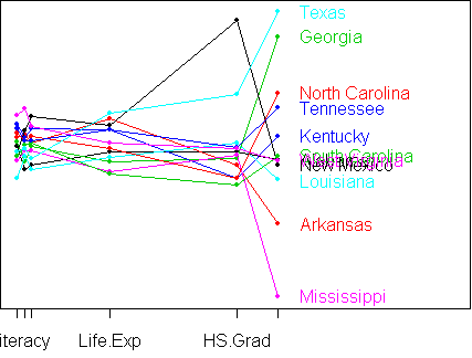
Are there any unusual states here? outliers suggests two:
> outliers(y,0.2)
                     D2   p.value
New Mexico     9.645276 0.1404071
West Virginia  9.399917 0.1523046
Since there are only a few variables in this dataset, we can examine
the outliers using a parallel-coordinate plot:
> parallel.plot(y)
axis reversed for Illiteracy Homocide
columns are -Illiteracy -Homocide Frost Life.Exp HS.Grad Income