Day 34 - Distances and transformations
Distance measures for nearest-neighbor
With numerical predictors, we found that Euclidean distance, after
appropriate rescaling, works well for nearest-neighbor classification.
What about categorical predictors? For one categorical predictor, a
natural metric is to say that two examples are similar if they have exactly
the same categorical value, and otherwise dissimilar. For multiple
categorical predictors, a natural generalization is to count the number of
disagreements between the predictor values for the two examples.
This is sometimes called Hamming distance.
But is this really the best distance? And what happens if we have both
numeric and categorical predictors?
The best metric that you can possibly use for
nearest-neighbor classification is this one:
d(x,z) = Pr(class(x) != class(z))
Intuitively, if we are going to choose z and assign his class to
x, then we should choose the z which is most likely
to have the correct class. It is almost tautological. But it does have
strong implications about which metrics you should use and which you should
stay away from.
As an example of what this rule implies, consider the case of one
categorical predictor, with values A, B, or C. Of the examples with value
A, 20% are in class 1. For value B, 90% are in class 1. For value C, 10%
are in class 1. Suppose we're using Hamming distance, with ties resolved
randomly. (If you don't like the idea of random tiebreaking, imagine there
are other predictors which add pseudo-random amounts to the distance.) To
classify an observation with value A, we pick a random example with value
A. The probability that we will get the correct class for the observation
is 0.2*0.2 + 0.8*0.8 = 0.68.
Using the optimal metric, we can do better. The optimal metric gives us a
way of measuring distance between different categories. For example, it
says that d(A,B) > d(A,C), since observations labeled A and B
are unlikely to be in the same class. It also says that d(A,A) >
d(A,C). This is counterintuitive until you realize that the
probability that we will get the correct class for an A is 0.2*0.1 +
0.8*0.9 = 0.74 if we match it with a C, which is better than matching
with another A.
This technique also extends to numerical predictors. See the references below.
Quadratic transformation
Last time we saw that nearest-neighbor was considerably better at
classifying handwritten digits than logistic regression. Why did this
happen, and how can we make logistic regression better? It all has to do
with the assumption of a linear class boundary.
An important thing to realize about the digit problem is that we were
trying to separate a small class, the 8's, from a much bigger class, the
non-8's. In these situations, it isn't unusual for the smaller class to
sit entirely within the big class, like so:
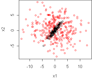
A linear boundary is therefore a bad assumption.
Besides handwritten digits, this "containment" situation also arises
in face detection
(classifying face images versus all other images)
and speaker detection (classifying sounds of a person's voice versus
all other sounds).
It doesn't happen so much with document classification, because usually
there are a few words which characterize the target class and none
others.
In a high dimensional dataset, where you can't make a scatterplot as above,
you can spot a containment situation
by making a predict.plot and seeing non-monotonic relationships
between the predictors and the class probability.
Here is the predict.plot for the digits dataset:
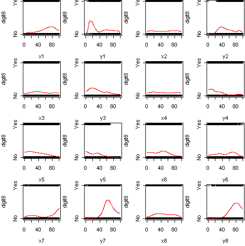
For many of these predictors, the class probability is not monotonic.
Sometimes it rises to a peak and then
falls again (see y7). This confirms that we have
containment.
In simple linear regression, we dealt with this sort of problem by making
transformations. It also works for logistic regression. A transformation
especially suited to handle containment is the quadratic
transformation. Instead of the model
p(y=1|x) = sigma(a + b1*x1 + b2*x2)
we will use
p(y=1|x) = sigma(a + b1*x1 + c1*x1^2 + b2*x2 + c2*x2^2 + b12*x1*x2)
The motivation for this is geometry: while a + b1*x1 + b2*x2 = 0
determines a line, a + b1*x1 + c1*x1^2 + b2*x2 + c2*x2^2 + b12*x1*x2 =
0
determines an ellipse.
Technically, the squared terms alone give an ellipse; the cross term
x1*x2 allows the ellipse to rotate.
To fit the quadratic model, we use the same logistic regression routine, just
with an enlarged set of predictors.
Here is the result for the example dataset above:
fit <- glm(y~x1+x2+I(x1^2)+I(x2^2)+x1:x2,frame,family=binomial)
cplot.knn(fit)
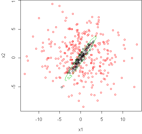
glm has trained the coefficients a,b1,b2,c1,c2,b12 to
give a snug ellipse around class 1.
Nearest-neighbor gives a similar, but bumpier, boundary:
> cplot.knn(fit)
> nn <- knn.model(y~.,frame)
> nn2 <- best.k.knn(nn)
best k is 3
> cplot(nn2)

This helps explain why nearest-neighbor was so much better on digits.
Here is the result on digits if we use this transformation:
# linear
> fit <- glm(digit8~.,x$train,family=binomial)
> misclass(fit)
[1] 162
> misclass(fit,x$test)
[1] 141

# quadratic, no cross terms
> fit2 <- glm(expand.quadratic(terms(fit),cross=F),x$train,family=binomial)
> misclass(fit2)
[1] 79
> misclass(fit2,x$test)
[1] 69

# quadratic
> fit2 <- glm(expand.quadratic(terms(fit)),x$train,family=binomial)
> misclass(fit2)
[1] 0
> misclass(fit2,x$test)
[1] 17

# nearest neighbor
> nn <- knn.model(digit8~.,x$train)
> misclass(nn,x$test)
[1] 8
The reduction in error is dramatic.
The function expand.quadratic has been used to automatically add
the extra terms. The linear fit has 17 coefficients, the quadratic with no
cross terms has 33, and the full quadratic has 152 coefficients. This
gives it enough flexibility to model the digit "8" class quite well.
But nearest neighbor is still better.
Gaussian kernel
Why are we still losing to nearest neighbor? In the
predict.plot above, we see that there is not just one
bump, but multiple bumps in the probability curves.
How can this happen? Take a look at these two examples of digit "8" in the
training set:
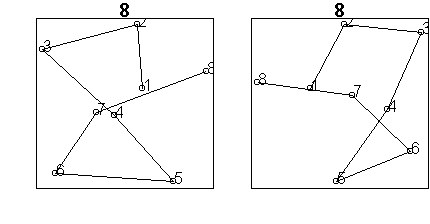
The digit on the left was drawn counterclockwise from the top, while the
digit on the right was drawn clockwise. Other examples start the stroke at
the top inside of the side. These seemingly minor changes have a large
effect in the predictor space: instead of x3 being small and
x8 large, we have x8 large and x3 small.
In the middle, we have other digits like "1". So the "8" class is not one
contiguous blob, as we have been assuming, but more like a collection of
blobs, separated by other digits. In such a situation, nearest-neighbor
has a distinct advantage because it only needs one example to represent
each possible drawing of "8".
There is a transformation which can help logistic regression in this
situation too: the Gaussian kernel transformation. We won't go into
the mathematics behind it but basically it is a parametric form of knn.
You can see some examples at the bottom of my Bayesian model
selection page. On that page, I discuss a method for choosing among
the different predictor transformations: linear, quadratic, or Gaussian
kernel. The Bayesian method has some advantages over cross-validation.
Code
Functions introduced in this lecture:
References
The optimal metric for nearest-neighbor is discussed in more detail in the
paper "Distance measures as prior probabilities".
Tom Minka
Last modified: Wed Apr 26 09:49:14 GMT 2006