Day 21 - Classification trees

Recursive partitioning can also be applied to predicting a categorical response, as in classification. We repeatedly select the most relevant predictor variable and use it to stratify the data. The resulting stratification maximizes the predictability of the response, e.g. our ability to classify the object. From now on, "response" and "class" will be used interchangeably.

For each categorical predictor, we can form a two-way contingency table relating it to the class variable. If the chi-square statistic of this table is small, then the predictor gives little information about the class: they are nearly independent. If the chi-square is large, then the predictor gives a lot of information about class. So we want to find the tables with large chi-square. Furthermore, as in regression trees, each split will be binary. So we need to merge predictor values (rows of the table) until only two remain. We already have a routine to do this: merge.table.

For a numerical predictor x, we exploit the fact that exactly two bins are required and simply search over all thresholds t such that the categorical variable x < t, x > t has large dependence on the class. This is also done with a chi-square test.

The resulting algorithm: for each predictor, abstract into two bins. Choose the abstracted predictor with largest dependence on the class. Stratify and recurse.

Classification trees are useful in data mining because they find the relevant variables and they are concise. They don't give precise predictive probabilities, however. We will discuss techniques for that later.

Mushroom classification

The illustrate the method, consider the following dataset of 5416 mushroom varieties, listing 22 categorical attributes as well as the "class" (edible or poisonous). Here is the first row:

 
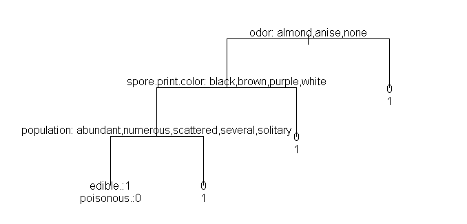
  cap.shape cap.surface cap.color bruises odor gill.attachment gill.spacing gill.size gill.color stalk.shape
1    convex     fibrous       red bruises none            free        close     broad     purple    tapering
  stalk.root stalk.surface.above.ring stalk.surface.below.ring stalk.color.above.ring stalk.color.below.ring
1    bulbous                   smooth                   smooth                   gray                   pink
  veil.type veil.color ring.number ring.type spore.print.color population habitat   class
1   partial      white         one   pendant             brown    several   woods edible.

Here is the resulting classification tree:

> tr <- tree(class~.,x)
> tr
node), split, n, yval, (yprob)
      * denotes terminal node

1) root 3803 edible. ( 0.623192217 0.376807783 )  
  2) odor: almond,anise,none 2420 edible. ( 0.979338843 0.020661157 )  
    4) spore.print.color: black,brown,purple,white 2379 edible. ( 0.996216898 0.003783102 )  
      8) population: abundant,numerous,scattered,several,solitary 2370 edible. ( 1.000000000 0.000000000 ) *
      9) population: clustered    9 poisonous. ( 0.000000000 1.000000000 ) *
    5) spore.print.color: green   41 poisonous. ( 0.000000000 1.000000000 ) *
  3) odor: creosote,foul,musty,pungent 1383 poisonous. ( 0.000000000 1.000000000 ) *
> plot(tr,type="uniform"); text(tr,pretty=0,label="yprob")

The algorithm has found a perfect and concise partitioning of the data. Each stratum contains varieties of a single class. This classifier has the form of an "OR" rule: if a mushroom has a foul odor OR it has green spores OR it appears in clusters, then it is poisonous.

Fisher's iris data

Another classic example is Fisher's dataset of iris flowers. It contains petal and sepal measurements of three different species: (sepals are the protective covering beneath the petals)

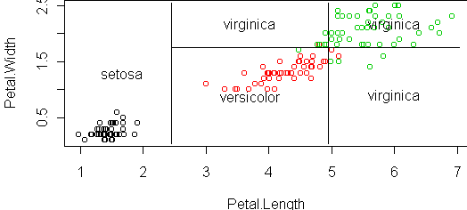
> iris[1:5,]
Sepal.Length Sepal.Width Petal.Length Petal.Width    Species
         6.4         2.8          5.6         2.2  virginica
         5.8         2.7          3.9         1.2 versicolor
         5.7         2.5          5.0         2.0  virginica
         5.5         2.4          3.8         1.1 versicolor
         5.6         2.9          3.6         1.3 versicolor
         ...
> tr <- tree(Species ~., iris)
> plot(tr,type="uniform"); text(tr,pretty=0,label="yprob")

Notice that the split on Sepal.Length has no effect on the dominant class; both leaves favor versicolor. But the algorithm makes a split anyway because the distribution of the classes, and consequently the confidence in the classification, is different between them.

To get a picture of what is going on, we can focus on Petal.Length and Petal.Width:

tr <- tree(Species ~ Petal.Length+Petal.Width, iris)
cplot(tr)

We see that setosa is a separate group whereas virginica and versicolor and partially confused using these measurments alone. The tree makes extra splits to separate border regions where there is a lot of confusion from interior regions which are well-defined.

Simple example of numerical predictor

Here is a distilled example of what happens with a numerical predictor. Suppose there is only one predictor, and the probability of class 2 gradually increases as you move along its domain. The first cut will be halfway through the domain, and further cuts will separate regions with different class probabilities:

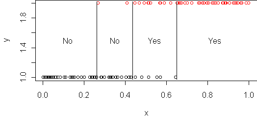
x <- sort(runif(100))
y <- x+rnorm(100)/10
y <- factor(y > 0.5)
levels(y) <- c("No","Yes")
tr <- tree(y~x)
cplot(tr)

Predicting churn

For a more complex example, consider the problem of predicting whether a long-distance phone customer will switch to another company ("churn"). The dataset we will work with describes 18 monthly statistics of 3333 customers, including whether they churned or not. Here is the first row:

  acct.len area intl vmail vmail.msgs day.mins day.calls day.charge eve.mins eve.calls eve.charge night.mins
1      128  415   no   yes         25    265.1       110      45.07    197.4        99      16.78      244.7
  night.calls night.charge intl.mins intl.calls intl.charge svc.calls churn
1          91        11.01        10          3         2.7         1    No

Some of these predictors are categorical and some numeric. Here is the resulting tree:

tr <- tree(churn~.,x)
plot(tr,type="uniform"); text(tr,label="yprob",pretty=0)

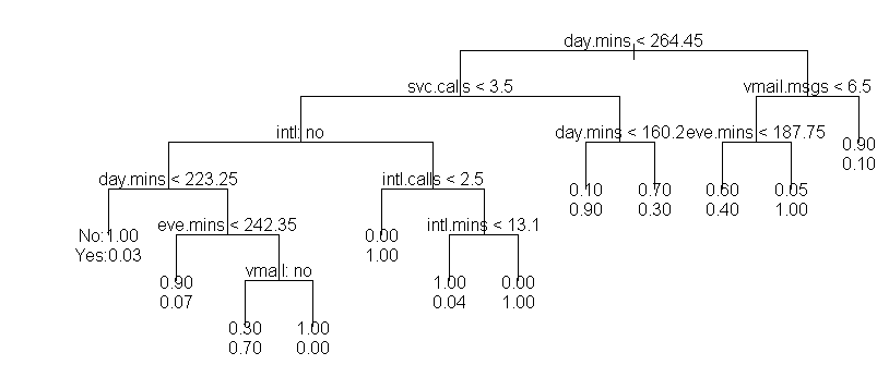
This classification scheme is quite sophisticated. Let's analyze it piece by piece.

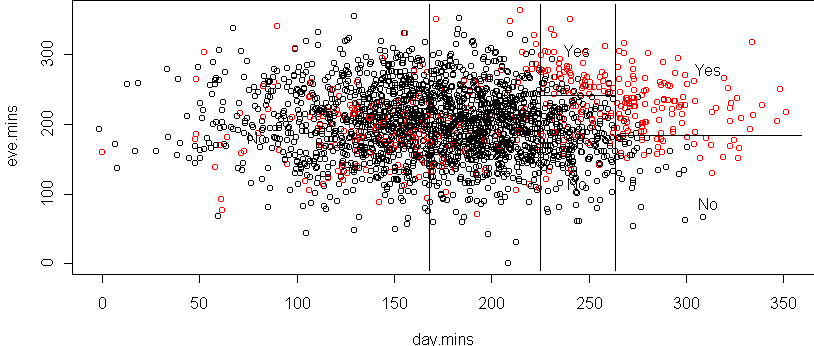
On the right side of the tree we see that people with a large number of daytime and evening minutes tend to churn, but only if they have a small number of voicemail messages. Here is the result of predicting churn only on day and evening minutes, restricted to those with a small amount of voicemail:

i <- (x$vmail.msgs < 6.5)
tr2 <- tree(churn~eve.mins+day.mins,x[i,])
cplot(tr2)

Strangely, there is not much association between day and evening minutes. But it is clear that customers with both a large number of day and evening minutes are more likely to churn (red). This is bad since these are the company's best customers.

In the middle of the tree we see that people who make many service calls yet have a small number of day minutes are likely to churn. These may be people who are just setting up their accounts. Here is a tree using only these two variables:

tr2 <- tree(churn~svc.calls+day.mins,x)
cplot(tr2)

There is clearly a change in churn above 3 service calls. The customers with the most minutes do not make many service calls.

On the left side of the tree we see an interaction between the number of international minutes vs. international calls. We can focus in on this interaction by building a tree for the data that fall under node 9:

y <- x[cases.tree(tr,"9"),]
tr2 <- tree(churn~intl.calls+intl.mins,y)
cplot(tr2)

There is quite a strong interaction here.

These plots are not just to check that the tree is correct. The idea is to use the tree as a springboard for a more detailed analysis that the tree cannot provide.

Background reading

A wealth of papers and software for classification and regression trees can be found at recursive-partitioning.com.

Tom Minka

Last modified: Mon Aug 22 16:34:09 GMT 2005