Day 18 - Merging numerical batches
Today we moved beyond purely categorical data into data where the response
variable is numerical. Numerical data is more difficult to handle
primarily because we have to make assumptions about the data distribution
that we didn't have to make with categories. The case of categorical
predictors for a numerical response requires the fewest assumptions so we
start with that. Later we will relate numerical predictors to numerical
responses, which requires a great deal of assumptions.
Properties of lift
The homework explores two properties of lift that we haven't talked about
before. The first property is the relation between lift and prediction
rules. A prediction rule is an implication of the form "A implies
B", such as "Giving birth implies being female" or "Being a veteran implies
being more than 5 years old". According to Boolean logic, "A implies B"
means that it is impossible (or very unlikely) for B to be false if A is
true. Note that if A is false then nothing is said about B.
The connection between lift and implication occurs when the lift is less
than 1: p(A|B)/p(A) < 1. This means that B reduces the
probability of A. In logical terms, we would write it as "B implies not A"
or "A implies not B" (these two statements are equivalent).
In general, you take one of the events involved in the lift calculation,
negate it, and make it the consequent of the implication.
It doesn't matter which event you negate: the logical meaning is the same
(and the lift is symmetric anyway).
If the lift between two events is greater than 1, no logical implication is
suggested. The lift of (birth,female) is greater than 1 since the
probability of giving birth increases when you know the person is female.
But you wouldn't say that being female implies giving birth.
The correct implication comes from the small lift of (birth,male)
(in fact the lift would be zero).
The second property of lift is that while lift is great at finding strong
associations, it doesn't always reflect the practical impact of an
association. Suppose two drugs interact in such a way that the probability
of an adverse event multiplies by five. If these drugs are rarely taken,
this may mean that 5 people had the adverse event as opposed to an expected
count of 1 person (nij/eij = 5). Compare that to a pair of
drugs which have a minor interaction but are frequently taken: nij =
11000, eij = 10000, nij/eij = 1.1. The second interaction
causes 1000 additional adverse events while the first only causes 4
additional events. For this reason, data miners sometimes prefer to use the
gain as a measure of the impact of an assocation.
Gain is the difference between actual and expected count: gain = nij -
eij. A confidence interval on the gain can be obtained from
the approximate standard error sqrt(nij), as used in the
confidence interval for lift.
Numerical batches
When you have categorical predictors for a numerical response, you
basically have a set of numerical batches, and the question is how do the
batches compare to each other. Let the categorical predictors be called
"factors", as in S. In introductory statistics, the only question of
interest when there is a single factor is whether the means are all equal.
This is called "one-way ANOVA", and is analogous to the chi-square test for
contingency tables. As in contingency tables, in this course we want to go
beyond this simple dichotomy and get an idea of how the batches vary.
In contingency tables, we went through four topics: visualization, sorting,
measuring deviations, and abstraction. For numerical batches,
visualization is handled by the boxplot. Sorting amounts to sorting the
batches by mean or median. Deviations from equality are measured using
contrasts, which are differences between means. The standard error
of a contrast is straightforward to compute and is given in Moore &
McCabe.
Abstraction means abstracting the categorical predictor to have fewer
values. For predictive abstraction, we want to merge values that predict
the same response, or equivalently we want to merge batches that have the
same distribution. Merging is based on a test of the similarity of the two
batches. To do this, we need to make assumptions about the distribution.
For this course, we will assume the batches are normal.
In introductory statistics, it is usual to assume that the the batches
have the same variance, i.e. our uncertainty in the response is the same
for all factor levels. In this case, comparing two batches
reduces to comparing their means. The canonical statistic for this is the
t-squared statistic whose formula is given below:
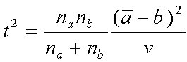
Here v is the variance of each batch, assumed to be the same for all batches.
Estimate v using (n1*v1 + n2*v2 + ...)/(n1+n2+...)
where vj is
the sample variance of batch j (I'm ignoring the
minus 1 correction that is sometimes used in the denominator).
Notice that the t-squared statistic for merging batches is the same as the
merging cost under Ward's method, because v is constant and can be ignored.
This means that t-squared merging is minimizing the same criterion that
Ward's is, namely the sum of squares.
However, the purpose of merging is to do data mining, so we typically do
not want to assume that the batches have the same variance. For this we
need a better criterion than the sum of squares. In particular, we need a
merging cost which takes into account the difference in variance as well as
the difference in means. If two batches have the same mean but different
variance, merging them can hide an important distinction.
An objective function which achieves this is the sum of log variances:
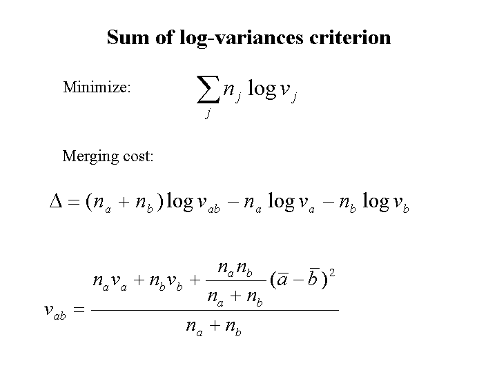
The merging cost does pay attention to the difference in means, but even if
the means are equal, the merging cost is not zero.
The merging cost is zero only when both means and both variances are equal.
This objective function, by the way, comes from Bayesian statistics and
is the marginal log-likelihood of the batches under the assumption of
normality. The sum of squares criterion is derived in the same way but
with an equal-variance constraint.
These two merging criteria are nicely illustrated by the time series
discussed on day17. Here it is again:
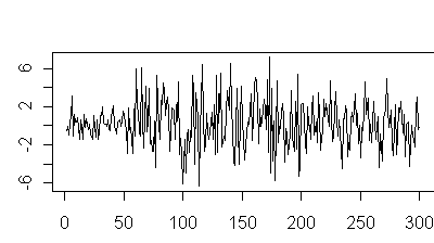
The mean of this time series doesn't change much, but its variance does.
Hence we would expect an equal-variance assumption to do poorly.
Ward's method gives breaks at 96 and 107, isolating the one period where
the mean seems to change.
The modified merging cost gives breaks at 52 and 199, corresponding to
the places where the variance changes:
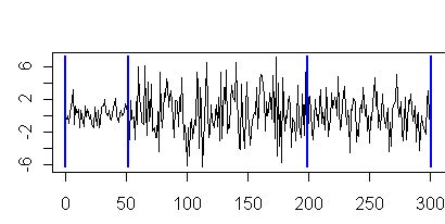
Unlike day17, we did not have to convert the data to a contingency table to
get this result, but we did have to assume normality within each segment.
Background reading
The connection between small lift and implication is discussed by Brin et
al, "Dynamic Itemset
Counting and Implication Rules for Market Basket Data". They also give
an efficient algorithm for finding associations with small lift.
Evaluating associations according to gain is described by Bay and Pazzani,
"Discovering and
Describing Category Differences: What makes a discovered difference
insightful?". They had human experts judge the importance of different
rules and found that the experts typically used gain as their criterion.
The Bayesian likelihood for normality is discussed in "Inferring a Gaussian distribution".
Tom Minka
Last modified: Tue Apr 25 09:53:05 GMT 2006