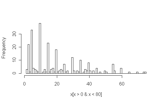
To make the plot readable, only the times greater than zero and less than 80 are shown. The command to do this is hist(x[x>0 & x<80],80). It appears that there are clusters around 10, 30, and 55 seconds.
According to museum theory, visitors tend to be either "busy", "greedy", or "selective". Busy visitors spend a small amount of time at each exhibit. Greedy visitors spend a lot of time at every exhibit. Selective visitors spend time at a small set of exhibits. It would be useful to classify visitors into these three types so that the museum can adapt its exhibits, either on a time-of-day or day-of-week schedule or dynamically as visitors move through the museum.
Time durations have been recorded for 45 visitors and 12 different exhibits, giving a data matrix with 45 rows and 12 columns. In this data, all cells have been filled in, but in practice we won't necessarily have time measurements for each visitor at all exhibits. How can we classify visitors?
The approach which has been adopted in the project is to use a histogram classifier. If we abstract the time durations into "zero" (0), "short" (S), and "long" (L), then we can make a three-bin probability histogram for each visitor class. A new visitor is classified by considering their exhibit times to be independent draws from one of the visitor class distributions.
The remaining question is how to define the abstractions "short" and "long". So far we have discussed three principles for abstraction: balance, beyond, and within. Balance alone is not appropriate since time is a numerical variable and differences in time are important. The beyond principle says that we should preserve distinctions between this data and other data we might get. In other words, it treats all 45 visitors we've seen as one group, and future visitors as another group. That does not fit the problem description either. The within principle is more reasonable, since we are trying to distinguish subgroups of the 45 visitors. Therefore we should consider clustering the times.
A histogram of all 45*12 = 540 time measurements is shown below.
To make the plot readable, only the times greater than zero and less than
80 are shown. The command to do this is
hist(x[x>0 & x<80],80).
It appears that there are clusters around 10, 30, and 55 seconds.
However, the unusual spiky structure of the histogram alerts us to possible
problems with this data. Lets zoom in to the times greater than zero and
less than 20:
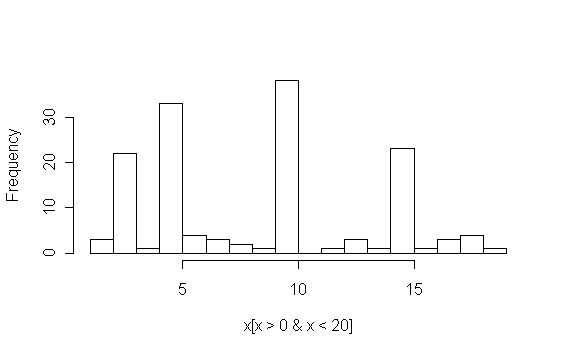
Apparently, some of the people recording the times rounded them to
multiples of five, and some did not. We wouldn't have known this without
looking at the data. The only way to fix this is to round all of the data
to multiples of five. This can be done with the command
round(x/5)*5.
Here is the histogram of rounded data:
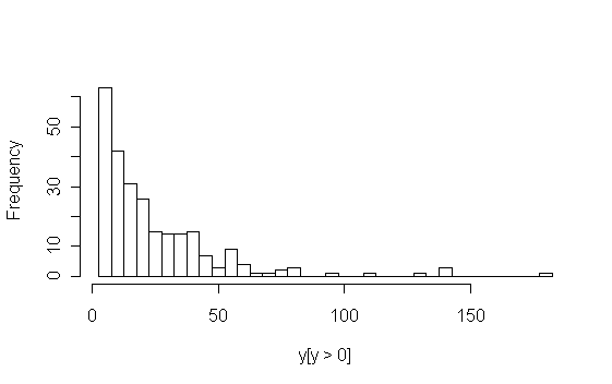
Now the interpretation is quite different.
To cluster this data, we can use Ward's method, via
break.hclust.
From the merging trace, 5 clusters are indicated.
Here is the result for 5 clusters:

The breaks are at 7, 27, 52, and 120.
Notice how there is a break at 120, even though the data is sparse there.
This is because the data is extremely spread out at the high end.
The break at 27 comes first in the hierarchy, so to answer the question
with two bins, "short" is less than 27 and "long" is greater than 27.