Asymmetrical Frequency Modulation (AFM)
Spectra
In order to be able to study the spectral behaviour of AFM, we first have to determine the spectral lines generated by AFM using equation 3.11 which is the spectral equation for AFM. This was done by writing a program in the C language [29][30] and running the program on a Silicon Graphics IRIS 4D workstation with a TEKTRONIX [31] graphics terminal.
Figure 4.1 shows the Pascal-like pseudo-code algorithm for implementing equation 3.11. A C language program was written to generate the Bessel function Jn(I) [32] and store it in a file, so that it could be referenced by the program computing the AFM spectrum.
Before the start of the C program, AFMSPRT.C, which is the main program, the variables runningN, freqA and ampA are declared. The variables freqA and ampA are used to store the calculated frequency components and amplitudes of equation 3.11 temporarily. The variable runningN is the running index that represents n in equation 3.11.
The constants minN and maxN, represent -n and +n
respectively. In equation 3.11, the index n actually runs from
-
* to +
*. However, in the computer, we cannot have
-
* or +
*. Therefore, minN and maxN are some
numbers that are large enough so that the calculated AFM spectrum is accurate.
Knowing that value of the Bessel function will rapidly decrease with increasing
order, we have chosen these indices to be about 12. To be more certain, we have
also test generated the Bessel function with index n equals to -12 and
+12. The calculated absolute values of the Bessel function are smaller than
10-8.
An array, i.e. reserved memory in the computer, is declared to store the calculated amplitudes for the respective frequency components. Its size is determined by the a constant MaxFreqToPlot, which is the highest frequency component we want plotted on the graphics screen of the computer.
The Bessel function generated by another program and stored in a file is also read into the computer memory as a look up table so that the calculation of the amplitudes of the various frequency components can be done very quickly.
From the START of the C program, we let the index runningN run from minN to maxN to create a loop. Within this loop, freqA is the calculated frequency component and ampA is the calculated amplitude of the current freqA. FreqA is then examined to see if it holds a negative value. If the calculated frequency is a negative value, then the frequency is inverted to become a positive value and the amplitude is also inverted to become an opposite signed value. This operation represents the reflection of frequency components from the negative frequency region about the 0 Hz axis into the positive frequency region. The amplitude ampA is then added into the array array(freqA). This is to allow the same frequency component calculated from other values of runningN to be added.
When the index runningN has finished running, i.e. reached maxN, the program exits from the loop and will start plotting the calculated frequency components as vertical lines on the TEKTRONIX [31] computer graphics screen . The length of the line represents the calculated amplitude of that frequency component. Negative amplitudes are plotted as vertical lines in the positive region of the amplitude axis but with a different colour. The amplitudes are also saved in a file for future reference.
START
Run the index runningN from minN to maxN
{
freqA = freqCarrier + runningN * freqModulator
ampA = bessel1(runningN,index)
If freqA is negative then invert the sign of freqA and ampA
Add ampA into array(freqA)
}
Plot the values in array(0) to array(MaxFreqToPlot) onto the graphics screen
END
In the listing of BESSEL.H in appendix 1, we have defined several subroutines to handle the special cases when calculating the Bessel function. The subroutine power(base,exponent) is a modified version of the built-in function pow(base,exponent) of the C language. The built-in version pow(base,exponent) will give rise to an error when both the base and exponent are equal to zero. Since the value of 00 is 1, we have modified power(base,exponent) to give a value of 1.0 when both base and exponent are zero. Other non-zero values of base and exponent are handled directly by the built-in pow(base,exponent) function of the C language.
In order to calculate the factorial of an integer, we have also defined a subroutine called factorial(arg1) where arg1 is an integer argument of the factorial function. This is because the factorial function is not a built-in subroutine of the C language.
The subroutines power(base,exponent) and factorial(arg1) are used by another subroutine named bessel1(n,x) which actually calculates the Bessel function. The arguments n and x are the order and the argument of the Bessel function respectively. The Bessel function is calculated based on the finite series :
![]()
where the argument p in the finite series is the argument n of the subroutine bessel1 and the argument x in the finite series is the argument x of the subroutine bessel1.
The series runs from n = 0 to
*. However, the value
* is not possible in a computer. We have therefore used a large
value of 150. The n in the series is represented by r in the
subroutine. We then have r running from r = 0 to 150 to calculate
the Bessel function. Since the denominator n! (p + n)! will be very much
greater than the numerator in the finite series, 150 is a sufficiently large
value.
The listing of the TEKTRONIX 4014 [31] graphics screen plotting subroutine in TEK4014.H contains the characters and symbols used to plot points and symbols on the TEKTRONIX screen. The TEKTRONIX screen has a resolution of 4096 by 3200 and the definition of a point or pixel on the screen must be translated from x,y coordinates to a set of ASCII characters. The terminal we used as a TEKTRONIX graphics terminal is a personal computer that has a program that is able to interpret the special characters and draw the points and lines on the screen. The personal computer emulates the TEKTRONIX graphics terminal by switching its monitor from text mode which only displays letters and numbers to graphics mode which is able to display graphics as well as letters and numbers. The resolution of the personal computer graphics screen is only 640 by 480. Therefore the 4096 by 3200 TEKTRONIX resolution is scaled down to 640 by 480 pixels. To view the full TEKTRONIX resolution, the personal computer can let us view part of the full 4096 by 3200 pixels at any time.
Appendix 2 is the listing for the AFM spectra generating program AFMSPRT.C which is the realization of equation 3.11 (AFM).
Let us now take a look at the spectral behaviour for different values of r. For example, if we set fc = 1000 Hz, fm = 100 Hz and I = 2, the value of r is varied from 0.4 to 4.0. The spectral plots with these AFM parameters are shown in figures 4.2 to 4.23.
We can see that as r is increased, the envelope of the spectrum drifts from left to right which explains the advantage of AFM over conventional FM. Because of this, the AFM spectrum is asymmetrical about the carrier frequency, unlike the FM spectrum. The peak of the envelope coincides with the carrier frequency when r reaches 1.0, i.e. where AFM becomes FM, another advantage of the AFM method. When r becomes greater than 1.0, the power gets shifted to the right side of the carrier frequency and the lower harmonics become diminished.
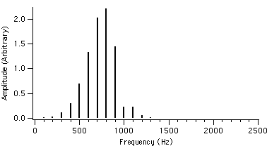
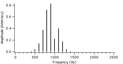
Figure 4.2 : fc = 1000 Hz I = 2 Figure 4.5 : fc = 1000 Hz I = 2
fm = 100 Hz r = 0.4 fm = 100 Hz r = 0.7
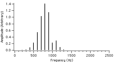
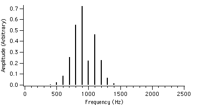
Figure 4.3 : fc = 1000 Hz I = 2 Figure 4.6 : fc = 1000 Hz I = 2
fm = 100 Hz r = 0.5 fm = 100 Hz r = 0.8
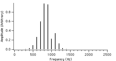
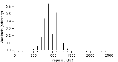
Figure 4.4 : fc = 1000 Hz I = 2 Figure 4.7 : fc = 1000 Hz I = 2
fm = 100 Hz r = 0.6 fm = 100 Hz r = 0.9
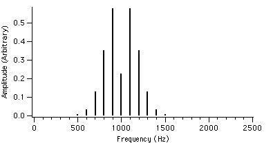
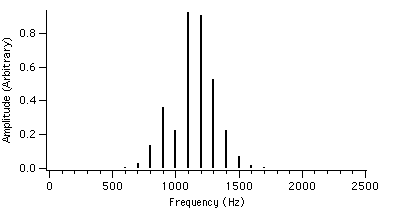
Figure 4.8 : fc = 1000 Hz I = 2 Figure 4.11 : fc = 1000 Hz I = 2
fm = 100 Hz r = 1.0 fm = 100 Hz r = 1.6
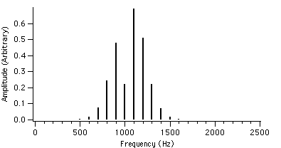
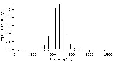
Figure 4.9 : fc = 1000 Hz I = 2 Figure 4.12 : fc = 1000 Hz I = 2
fm = 100 Hz r = 1.2 fm = 100 Hz r = 1.8
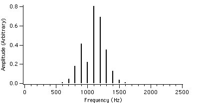
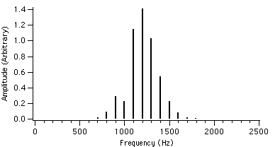
Figure 4.10 : fc = 1000 Hz I = 2 Figure 4.13 : fc = 1000 Hz I = 2
fm = 100 Hz r = 1.4 fm = 100 Hz r = 2.0
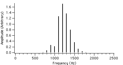
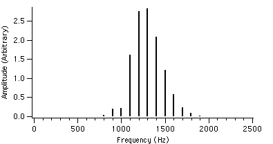
Figure 4.14 : fc = 1000 Hz I = 2 Figure 4.17 : fc = 1000 Hz I = 2
fm = 100 Hz r = 2.2 fm = 100 Hz r = 2.8
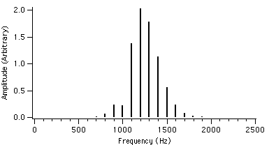
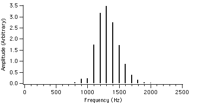
Figure 4.15 : fc = 1000 Hz I = 2 Figure 4.18 : fc = 1000 Hz I = 2
fm = 100 Hz r = 2.4 fm = 100 Hz r = 3.0
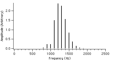

Figure 4.16 : fc = 1000 Hz I = 2 Figure 4.19 : fc = 1000 Hz I = 2
fm = 100 Hz r = 2.6 fm = 100 Hz r = 3.2
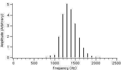
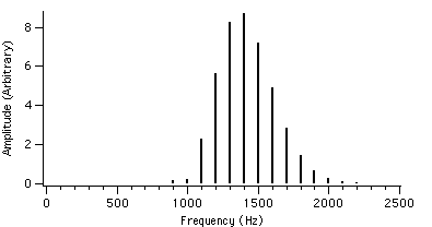
Figure 4.20 : fc = 1000 Hz I = 2 Figure 4.23 : fc = 1000 Hz I = 2
fm = 100 Hz r = 3.4 fm = 100 Hz r = 4.0

Figure 4.21 : fc = 1000 Hz I = 2
fm = 100 Hz r = 3.6
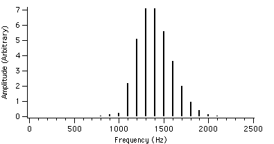
Figure 4.22 : fc = 1000 Hz I = 2
fm = 100 Hz r = 3.8