Contents

clc
close all
clear all

Key-Take Away

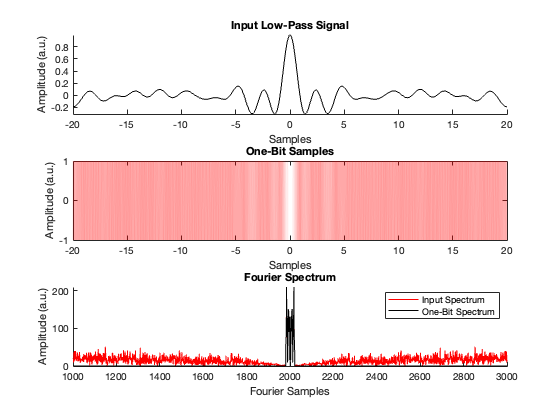
For low-pass signals, one-bit sampling via sigma-delta quantization
enables to retain the input signal features in the Fourier domain via
noise shaping.

Key Reference
 * Approximating a bandlimited function using very coarsely quantized
data by Ingrid Daubechies and Ron DeVore (Annals of Mathematics, 2003)

This can further be extended to sparse signals, for instance, see:

Function Definitions

ft = @(x) fftshift(fft(x));
K = @(x) sinc(x);


% Implement Sigma Delta Quantization Routine
% Self-Containted Matlab Function

function [q u] = SDQ(data);
data = data(:);

d_iter = [0 ; data];
u      = zeros(1,numel(d_iter));
u(1) = 0.9;

for k  = 2:numel(d_iter);
    q(k)  = sign(u(k-1) + d_iter(k));
    u(k) = u(k-1) + d_iter(k) - q(k);
end

v =0;
q(1) = [];

end

Define Low-Pass Signal

% Sampled Time Vector
t  = -20:0.01:20; t = t(:);

% Create Exact Low-Pass Window
LPF_window = K(t);
LPF_F = fft(LPF_window);
LPF_F(abs(LPF_F)<= 0.2.*max(abs(LPF_F)))=0;


% Randomize Fourier Amplitudes
Z = rand(numel(t),1) + 0i.*rand(numel(t),1);

% This creates an exactly low-pass function (no spectral leakage) with
% random Fourier amplitudes.
F = LPF_F.*Z;
f = real(ifft(F));
f = f./max(abs(f));
f = f-mean(f);

Perform One-Bit Measurements via Sigma-Delta Quantization

q = SDQ(f);

% Define Fourier Transforms via FFT
F = ft((f));
Q = ft(q);

Plot results

close all
subplot(3,1,1)
plot(t,f,'k')
axis tight
title('Input Low-Pass Signal')
xlabel('Samples')
ylabel('Amplitude (a.u.)')
box off


subplot(3,1,2)
plot(t,q,'Color',[1 0 0 0.05],'LineWidth',1)
title('One-Bit Samples')
xlabel('Samples')
ylabel('Amplitude (a.u.)')



subplot(3,1,3)
hold on;
plot((abs(Q)),'r')
plot((abs(F)),'k')
axis tight
xlim([1000 3000])
title('Fourier Spectrum')
xlabel('Fourier Samples')
ylabel('Amplitude (a.u.)')
legend('Input Spectrum', 'One-Bit Spectrum')