ReproduceResult

Plot original signal vs. modulo samples

clc
close all
clear all
set(0, 'DefaultLineLineWidth', 2);

% Load the 8kHz sampled dataset
load Data_8k.mat


% Define Fourier Transform magnitude function in dB
FT = @(x) db(abs((fft(x))));

% Set parameters for the reconstruction algorithm
lambda = 0.4;          % Regularization parameter
Ts = 1e-5;             % Sampling period (100 kHz sampling rate)
t = 0:Ts:(numel(x)-1)*Ts;  % Time vector
c1 = [1 1 1] .* 0.7;   % Gray color definition for plotting




% Recover signal using Unlimited Sampling Reconstruction algorithm
rec = US_Rec(y, x, lambda, 4);

Plot original signal vs. modulo samples

figure(1);
subplot(3,1,1);
hold on;
plot(t, x, 'Color', c1);
stem(t, y, 'r', Marker='none', LineWidth=2);
axis tight;
legend('Conventional ADC', 'MADC', 'Location', 'northeast', 'Orientation', 'horizontal', 'Box', 'Off');
ylim([-2 3]);
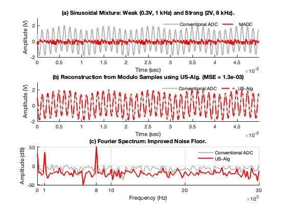
title('(a) Sinusoidal Mixture: Weak (0.3V, 1 kHz) and Strong (2V, 8 kHz).');
ylabel('Amplitude (V)');
xlabel('Time (sec)');

% Plot original signal vs. reconstructed signal
subplot(3,1,2);
hold on;
plot(t, x, 'Color', c1);
plot(t, rec - mean(rec) + mean(x), 'r-.', 'LineWidth', 2);
axis tight;
legend('Conventional ADC', 'US-Alg', 'Location', 'northeast', 'Orientation', 'horizontal', 'Box', 'Off');
ylim([-2 3]);
str = sprintf(['(b) Reconstruction from Modulo Samples using US-Alg. (MSE = %0.1e)'], immse(x, rec));
title(str);
ylabel('Amplitude (V)');
xlabel('Time (sec)');

% Plot frequency spectrum comparison
subplot(3,1,3);
N = numel(x);
f = ([0:N-1]) / N / Ts;
hold on;
plot(f, FT(x), 'Color', c1);
plot(f, FT(rec), 'r');
axis tight;
legend('Conventional ADC', 'US-Alg', 'Box', 'off');
xlim([0 30] .* 1e3);
title('(c) Fourier Spectrum: Improved Noise Floor.');
ylabel('Amplitude (dB)');
xlabel('Frequency (Hz)');
xticks(union(0:10:30, [1 8]) .* 1e3);
grid on;

% Adjust the exponent of the frequency axis for clarity
ax = gca;
ax.XAxis.Exponent = 3;

Contents

Plot original signal vs. modulo samples