Bayesian model selection
Tom Minka
 Bayesian model selection uses the rules of probability theory to select
among different hypotheses. It is completely analogous to Bayesian
classification. It automatically encodes a preference for simpler, more
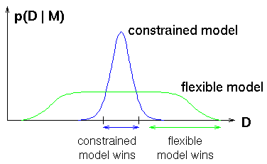
constrained models, as illustrated at right. Simple models, e.g. linear
regression, only fit a small fraction of data sets. But they assign
correspondingly higher probability to those data sets.
Flexible models spread themselves out more thinly.
The probability of the data given the model is computed by integrating
over the unknown parameter values in that model:

which reduces to a problem of calculus. This quantity is called the
evidence for model M.
Specific examples of computing the evidence follow.
A useful property of Bayesian model selection is that it is guaranteed to
select the right model, if there is one, as the size of the dataset grows
to infinity.
Polynomial fitting
A central issue in polynomial fitting is selecting the degree of the
polynomial. To do this, we compute the probability of the data for each
possible degree. For a given degree, this requires integrating over all
possible polynomial fits, which can be done analytically.
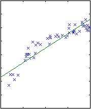
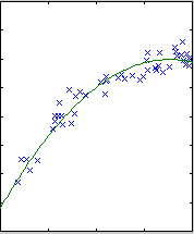
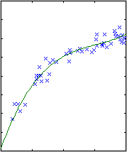
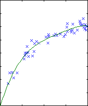
The results are shown below.

| 
| 
|
| degree 1
| degree 2
| degree 3
|

| 
| 
|
| degree 4
| degree 5
| degree 6
|

|
| 
|
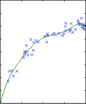
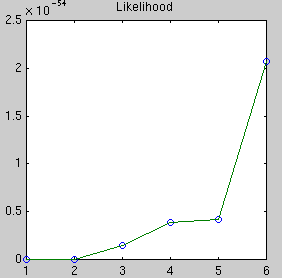
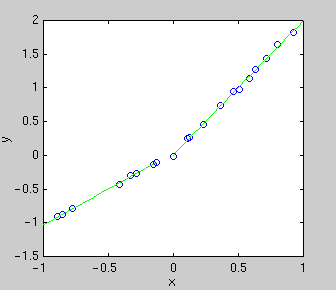
The likelihood only considers the single most probable curve, as shown for
each degree. The likelihood is the negative squared-error of the fit. It
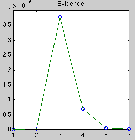
always increases with increasing degree. But the evidence reaches a
maximum at degree 3, which happens to be the true degree in this case. The
data is much more likely to have arisen from a third-degree polynomial than
a high-degree polynomial which just happened to look third-degree.
The same procedure works for regression with splines, radial basis
functions, and feedforward neural networks. See my paper "Bayesian linear regression".
Changepoint analysis
A changepoint model allows different parts of a dataset to obey different
probability laws. For example, all data received before time t
follows model A, while data received after time t follows model
B. A central issue is determining the number of changepoints. The
likelihood is not sufficient for this purpose because it will always prefer
more changepoints. We can use Bayesian model selection by computing the
probability of the data for each number of changepoints. For each number
of changepoints, we need to integrate over all possible changepoint
positions and all sub-models given those changepoints.
This technique is described in my paper
"Bayesian linear regression".
This is actually quite simple mathematically since the integral over
changepoint positions is a discrete sum. For example, consider a linear
regression changepoint model. The integral over possible lines was solved
in the curve fitting problem. Now we sum that quantity over possible
changepoints. Here are two examples:

| 
|

| 
|
| Evidence for each changepoint
| Evidence for each changepoint
|
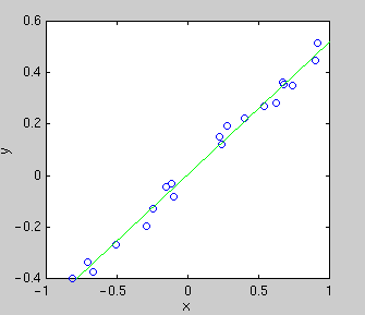
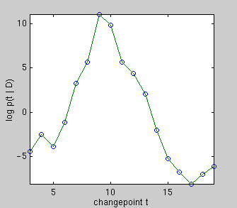
On the left, there really is a changepoint at t = 9. Plotted underneath is
the evidence for each changepoint position, which is an integral over the
parameters of the two linear sub-models. Summing over all changepoint
positions gives the probability of the data given that there is one
changepoint. Comparing this to the evidence for zero changepoints,
i.e. the evidence for a single line, gives an
overwhelming probability of there being a changepoint.
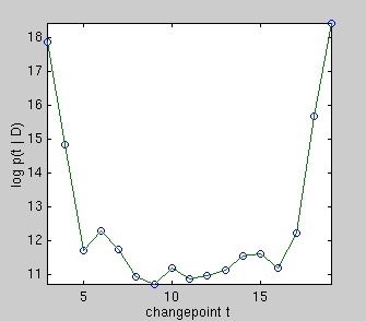
On the right, there really is no changepoint. Summing over all changepoint
positions gives a probability lower than that of a single line.
So we correctly infer that there is no changepoint.
Principal component analysis
Principal component analysis (PCA) decomposes high-dimensional data into a
low-dimensional subspace component and a noise component. This
decomposition is useful for data compression as well as de-noising, making
it a common first step for many data processing tasks. Here we use
PCA for density estimation, or equivalently lossless coding.
A central issue in PCA is choosing the dimensionality of the subspace
component so that all of the noise, but none of the signal, is removed. To
do this, we compute the probability of the data for each possible subspace
dimensionality. For a given dimensionality, this requires integrating over
all possible PCA decompositions, i.e. all possible subspaces. This can be
done analytically, but it is simpler to approximate it using Laplace's
method. Laplace's method essentially just measures the sensitivity of the
likelihood to each parameter (the parameters here are the basis vectors for
the subspace). Even simpler is the BIC method, which assumes the same
sensitivity to each parameter. Both are correct asymptotically.
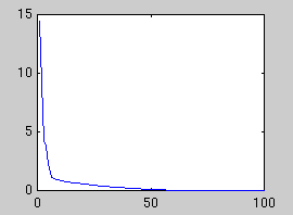
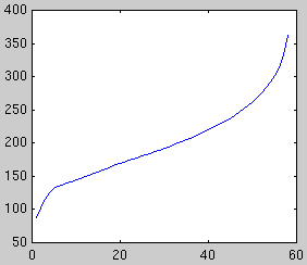
In the first example, a synthetic data set of 60 points in 100 dimensions
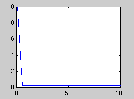
has been sampled. Below is plotted the eigenvalues of the true covariance
matrix and the observed covariance matrix. These measure the variance in
each dimension. The dimensions after 5 are good candidates for noise,
since they all have the same variance. The presence of a signal always
increases the variance above the noise floor, which we assume is constant.
| True eigenvalues
| Observed eigenvalues
|

| 
|
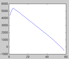
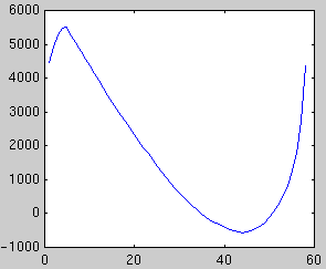
Next we plot the evidence for each subspace dimensionality, using Laplace's
method and BIC:
| Likelihood
| Laplace evidence
| BIC evidence
|

| 
| 
|
Both methods peak at dimensionality 5, however BIC is increasingly
unreliable for large dimensionalities. In some cases, the second peak may
exceed the first.
Cross-validation, a non-Bayesian model selection technique, also picks 5.
However it is far more costly to compute. The evidence approximations can be
computed directly from the eigenvalue spectrum and they are very fast.
See the paper "Automatic choice of dimensionality for PCA".
Classification
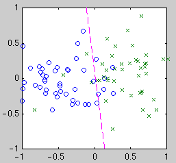
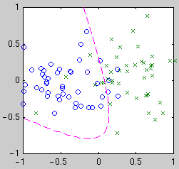
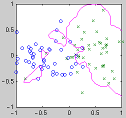
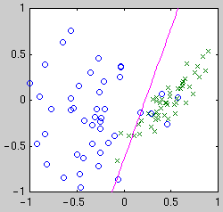
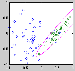
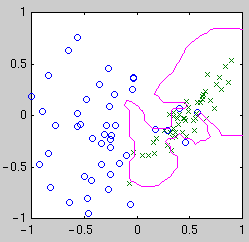
In classification we want to construct a function which takes in a
measurement and outputs c when the measurement is most likely to
be in class c. In other words, we want to construct boundaries
in measurement space which delineate the classes. Once we have chosen a
parametric form for the function, it is straightforward to find the
function which best fits training data. But there are many different
parametric forms to choose from and so we have a model selection problem.
If the classifier function is linear in the parameters, then the task
becomes similar to curve fitting as above. We still have the choice of
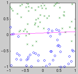
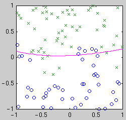
what basis functions to use. Consider three different bases: linear,
quadratic, and Gaussian kernel. Linear means our classifier function is
simply a weighted sum of the measurements---the boundary is a line.
Quadratic means the function is a quadratic function of the
measurements---the boundary is a parabola, hyperbola, or ellipse. Gaussian
kernel means our classifer function is a weighted sum of Gaussians
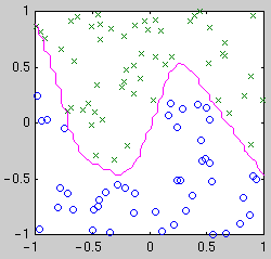
centered on the data points. Example classifiers are shown below.

| 
| 
|
| Linear
| Quadratic
| Gaussian kernel
|

| 
| 
|
| Linear
| Quadratic
| Gaussian kernel
|

| 
| 
|
| Linear
| Quadratic
| Gaussian kernel
|
Intuitively, we see that the "best" classifier in each case balances
simplicity against the need to fit the data. For Bayesian model selection,
we integrate over the possible classifier functions for each model.
Performing this integral is complicated by the fact that the likelihood of
a classifier function is not a smooth function of its parameters. The
likelihood is relatively constant until a data point becomes mislabeled,
when it goes down abruptly. Thus the integral has a combinatorial flavor.
In my PhD work, I developed a deterministic method for approximating this
integral which is faster than Monte Carlo methods. See
"Expectation Propagation for approximate
Bayesian inference".
Other problems
Bayesian model selection is useful for many other problems, such as
choosing the size of a mixture model or the structure of a Hidden Markov
Model. It has the potential to become a standard part of every analyst's
toolbox.
Further reading
Thomas P Minka
Last modified: Fri Sep 23 08:48:26 GMT 2005
 Bayesian model selection uses the rules of probability theory to select
among different hypotheses. It is completely analogous to Bayesian
classification. It automatically encodes a preference for simpler, more
constrained models, as illustrated at right. Simple models, e.g. linear
regression, only fit a small fraction of data sets. But they assign
correspondingly higher probability to those data sets.
Flexible models spread themselves out more thinly.

